Taylor Series Approximation of sin(x) in GeoGebra

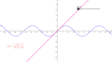
This example demonstrates how to approximate the trigonometric function sin(x) using its Taylor series and visually compares the approximation as the number of terms increases. It focuses on key ideas from calculus: Taylor (power) series expansion, finite-sum approximation of an infinite series, and convergence/accuracy of local polynomial approximations for a smooth function. The construction is implemented by building the partial sum with GeoGebra’s Sum command, using the objects g, n, f, and text2: n controls the truncation order (how many Taylor terms are included), f represents the resulting Taylor polynomial/approximation function, g provides the plotting or parameter setup, and text2 displays the corresponding formula or order information on the canvas. Suitable for high school to early undergraduate learners studying series, function approximation, and graph-based intuition in calculus.