Picard–Lindelöf Iteration When h(x,y) and h_y(x,y) Are Bounded and Continuous Ev

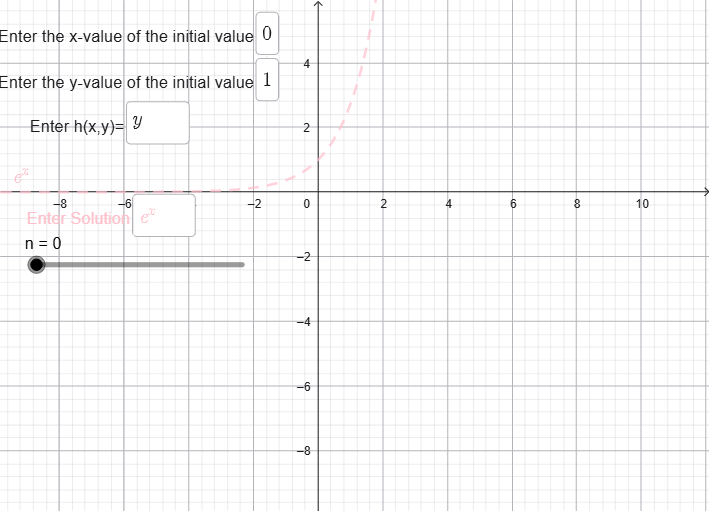
This GeoGebra example dynamically illustrates the Picard–Lindelöf iteration process for an ordinary differential equation, demonstrating that when the function h(x,y) and its partial derivative h_y(x,y) are bounded and continuous on the entire plane, the solution to the initial value problem exists not only locally but can be extended to the whole domain. The core mathematical concepts include the existence and uniqueness theorem for ODEs, Picard iteration sequences, uniform convergence, and the Lipschitz condition. The construction uses GeoGebra's Textfield and InputBox objects (InputBox1, InputBox2, InputBox3) to let users input initial conditions, the iteration number n, and the function h; the Integral command computes the integral expressions in each iteration step, generating a sequence of function objects f_1 through f_17 and corresponding g_1 through g_17 that progressively approximate the exact solution. This is suitable for university-level mathematics students studying differential equations, numerical analysis, or qualitative theory of ODEs, and also serves as a classroom demonstration for instructors to visualize the constructive proof of the existence and uniqueness theorem.