Numerical Damped Mass–Spring Response via ODE Solving

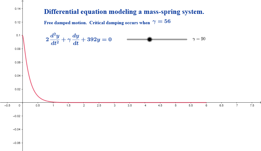
This example demonstrates how a damped mass–spring system vibrates and decays under different damping coefficients γ, visualized through solution plots and surface-style comparisons. It centers on a second-order linear ordinary differential equation with damping, connecting derivatives of the state variables to the system’s time response. Key construction choices include using GeoGebra’s SolveODE to compute the numerical solution, treating γ as a parameter, and employing numericalIntegral1 to obtain integral-based quantities used in the visualization or derived metrics. Additional text objects (text1–text4) annotate the equation, parameter values, and what each curve/surface represents. The example is well suited for instruction in differential equations, numerical methods, and mathematical modeling at the high-school advanced level and early university courses.