Series-Based Construction of Bessel Functions

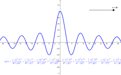
This example demonstrates how a Bessel function can be constructed numerically and visualized by using a series (summation) representation, highlighting its characteristic oscillatory behavior. The key mathematical ideas include Bessel functions, expressing special functions via infinite (or truncated) sums, and studying how parameters influence the resulting function values and graph shape. From the construction summary, the GeoGebra setup centers on the command Sum, summing over an index n to compute the desired expression from the involved objects (such as g and text2). The computed values are then used to produce the function graph so learners can observe the pattern and convergence behavior visually. Suitable for high-school advanced topics through early undergraduate learning, especially for lessons on series, functions, and graphing techniques.