Euler Method for ODE y'=x²+y² with Slope Field

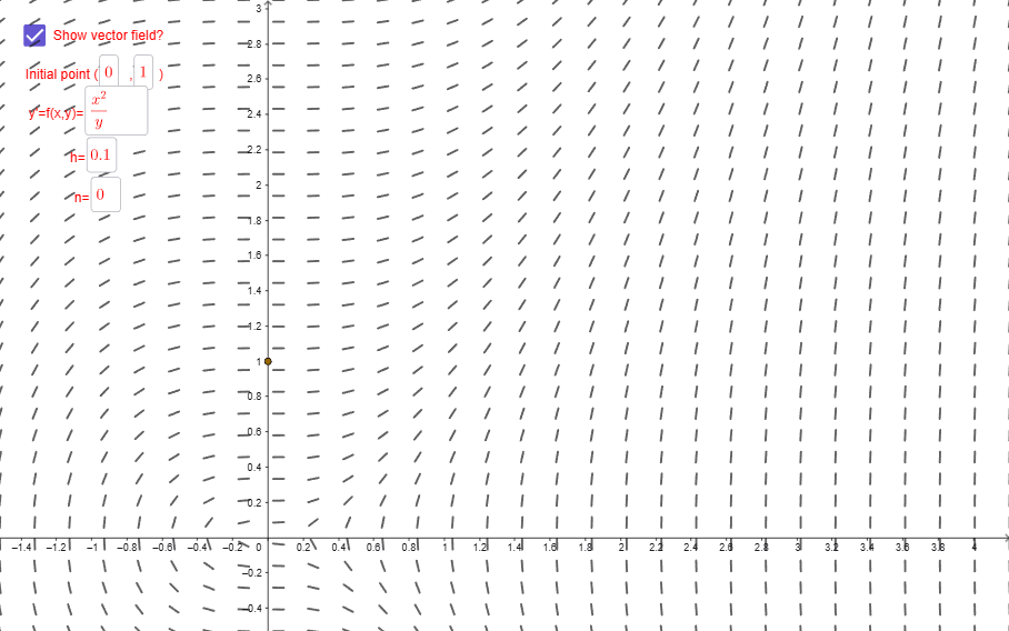
This example demonstrates the Euler Method for numerically solving the first-order ordinary differential equation y'=x²+y², visualized with a slope field. The core mathematical concepts include differential equations, numerical methods, slope fields, iterative approximation, and vector fields. Construction highlights: the SlopeField command generates the direction field, Textfield and InputBox objects allow interactive input of initial conditions (xinitial, yinitial) and step size h, Vector commands draw Euler iteration steps, and multiple points (A1~C9) and objects (a, b, n, f) trace the numerical solution path. Suitable for advanced high school or introductory college calculus students to explore how numerical solutions approximate the true solution and how step size affects accuracy.