Standardizing the Normal Distribution: Comparing X~N(μ,σ²) and Z~N(0,1)

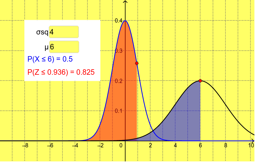
This GeoGebra example demonstrates the standardization of a normally distributed random variable X ~ N(μ, σ²) into the standard normal variable Z ~ N(0, 1), enabling side-by-side comparison of their probability density curves, shapes, positions, and areas under the curve. Core mathematical concepts include the normal distribution, Z-score standardization, probability density functions, definite integrals for probability areas, and the effects of mean μ and variance σ² on curve location and spread. The construction uses GeoGebra commands such as Point, Integral, Textfield, and Polygon, together with function objects f and g, parameter objects a, b, μ, σsq, and input controls inputBox1 and inputBox2 to create dynamic, interactive visualizations. It is suitable for high school advanced mathematics, university probability and statistics courses, and self-learners studying normal distribution standardization and graphical transformation.