
Frequency Polygon, Cumulative Frequency, and Box Plots
Loading the math board and drawing, please wait…
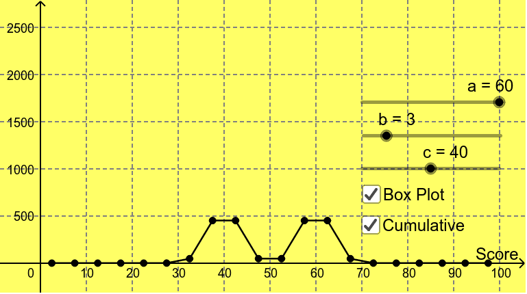
This example demonstrates the creation of frequency polygons, cumulative frequency distributions, and box plots by overlaying two normal distributions with means a and c, and standard deviations b and 3 respectively. Key math concepts include normal distributions, frequency polygons, cumulative frequency, box plots, mean, and median. GeoGebra commands used include Integral, Sequence, Intersect, BoxPlot, Point, Vector, and Textfield for construction. Suitable for high school students and educators in probability & statistics and data analysis.
GeoGebra Commands & Parameters
Integral(h) → pSequence(((5 * i) - 2.5, Integral[h, (5 * (i - 1)), (5 * i)]), i, 1, 20) → list1Sequence(Segment[Element[list1, i], Element[list1, i + 1]], i, 1, 20) → list3Sequence(((5 * (i - 1)), q((5 * i) - 5)), i, 1, 21) → list2Intersect(q, d, (49.99999999997028, 999.9999999999693)) → AIntersect(q, e, (40.0000000000929, 500.0000000254383)) → BIntersect(q, i, (60.00000000182589, 1500.000000229724)) → CIntersect(q, j, (30.128419806473982, 0.5000000005626362)) → DSequence(If[y(Element[list1, i]) < 1, 1, 0], i, 1, 20) → list4Intersect(q, k, (67.72748791064672, 1995)) → EBoxPlot(2500, 250, min, LQ, median, UQ, max) → lPoint(q) → FVector(G, F) → uVector(F, H) → vTextfield(a) → inputBox1Textfield(b) → inputBox2Textfield(c) → inputBox3
AI Drawing Prompt Reference
Draw frequency polygons, cumulative frequency distributions, and box plots for two normal distributions with means a and c, and standard deviations b and 3 respectively. First, calculate and plot the frequency polygons, then the cumulative frequency distributions, and finally overlay the box plots. Clearly show the relationships between means and medians, and label parameters a, b, c.
The prompt above was compiled from the original drawing commands and is for reference only.