
Continuity of a Piecewise-Defined Function
Loading the math board and drawing, please wait…
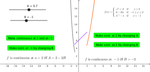
This example demonstrates the continuity of piecewise-defined functions across different intervals. Key math concepts include continuity, derivatives, and function graphing. It utilizes GeoGebra objects like A, B, f, g, h, p, q, r, buttons, and text elements for interactive exploration, suitable for high school calculus and function analysis.
GeoGebra Commands & Parameters
Numeric A(0.7)Numeric B(-1.0)f(x) = x^(2) + Ag(x) = 6 - (B * x)h(x) = 4^((-x)) - 1p(x) = If[2 ≤ x ≤ 100, f(x)]q(x) = If[-1 ≤ x ≤ 2, g(x)]r(x) = If[-100 ≤ x ≤ -1, h(x)]
AI Drawing Prompt Reference
Draw a single coordinate-plane graph for a piecewise-defined function using three interval pieces controlled by constants. First set constants A=0.7 and B=-1.0, then define the functions f(x)=x^2+A, g(x)=6-(B·x), and h(x)=4^(-x)-1. Next form three piecewise pieces: p(x)=f(x) for 2≤x≤100, q(x)=g(x) for -1≤x≤2, and r(x)=h(x) for -100≤x≤-1. Plot the curves of p, q, and r on their respective intervals, so the viewer can examine how the pieces connect at the boundaries and discuss continuity.
The prompt above was compiled from the original drawing commands and is for reference only.