
Normal Approximation to the Binomial Distribution by Gareth Daniels
Loading the math board and drawing, please wait…
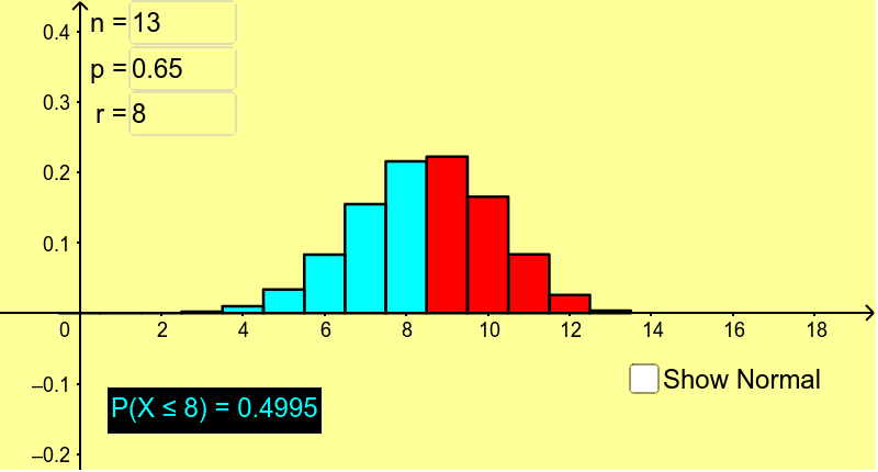
This example visually demonstrates how the normal distribution approximates the binomial distribution and the necessity of a continuity correction. It involves core math concepts like binomial distribution, normal distribution, continuity correction, and probability & statistics. Constructed using GeoGebra commands and objects such as BinomialDist, Sequence, Max, Normal, BarChart, Integral, and Textfield. Suitable for high school and above learners to understand distribution approximation and correction in probability statistics.
GeoGebra Commands & Parameters
BinomialDist(n, p) → aSequence(((Binomial[n, i] * p^(i)) * (1 - p)^(n - i)), i, 0, n) → list1Max(list1) → bBinomialDist(n, p) → cNormal((n * p), sqrt(((n * p) * (1 - p))), x) → fSequence(i, i, 0, r) → list2Sequence(Element[list1, i], i, 1, r + 1) → list3BarChart(list2, list3) → dIntegral(f, -100, r) → eIntegral(f, -100, r + 0.5) → gTextfield(n) → inputBox1Textfield(p) → inputBox2Textfield(r) → inputBox3
AI Drawing Prompt Reference
Create a visual comparison of a binomial distribution and its normal approximation. Draw a bar chart representing the binomial probability mass function for a given number of trials and success probability, with bars at each integer success count. Overlay a smooth normal distribution curve with the same mean and standard deviation. Mark a cutoff value on the x-axis, and shade two areas under the normal curve: one from negative infinity to the cutoff, and another from negative infinity to the cutoff plus 0.5, to illustrate the continuity correction. Include three input fields to adjust the number of trials, success probability, and cutoff value, with the graph updating dynamically.
The prompt above was compiled from the original drawing commands and is for reference only.