
Demonstrating Continuous Models for Discrete Random Variables
Loading the math board and drawing, please wait…
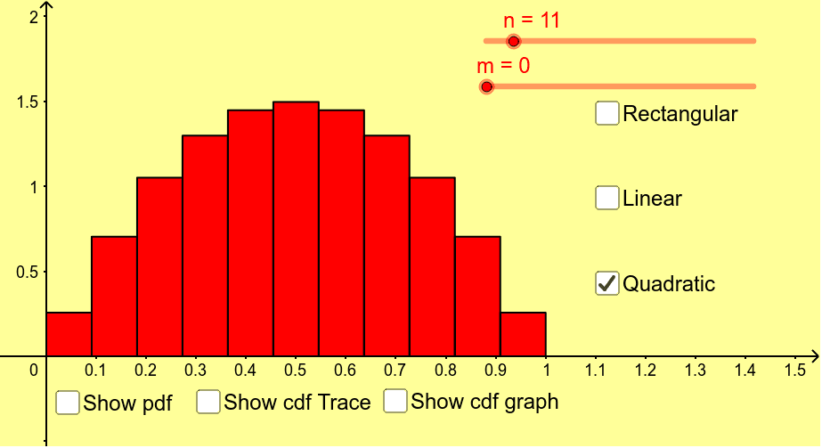
This example illustrates how discrete random variables can be better modeled using a continuous approach. It involves core math concepts like Probability Density Functions, Distributions, Statistical Characteristics, and Linear Regression. GeoGebra commands and objects used include Function, Sequence, and BarChart for constructing the visualizations. Suitable for high school and above students, or educational purposes needing to understand continuous probability models.
GeoGebra Commands & Parameters
Function(1, 0, 1) → fFunction(-2 * x + 2, 0, 1) → gFunction(-6 * x * (x - 1), 0, 1) → hSequence(n * Integral[h, i / n, (i + 1) / n], i, 0, n - 1) → intshBarChart(0, 1, intsh) → charthSequence(n * Integral[g, i / n, (i + 1) / n], i, 0, n - 1) → intsgSequence(n * Integral[f, i / n, (i + 1) / n], i, 0, n - 1) → intsfBarChart(0, 1, intsg) → chartgBarChart(0, 1, intsf) → chartfBarChart(0, 1, intsf) → chartfborBarChart(0, 1, intsg) → chartgborBarChart(0, 1, intsh) → charthborSequence(Element[intsf, i], i, 1, n * m) → intsfmBarChart(0, m, intsfm) → chartfmBarChart(0, m, intsfm) → chartfmborSequence(Element[intsg, i], i, 1, n * m) → intsgmSequence(Element[intsh, i], i, 1, n * m) → intshmBarChart(0, m, intsgm) → chartgmBarChart(0, m, intshm) → charthmBarChart(0, m, intshm) → charthmborBarChart(0, m, intsgm) → chartgmborSequence((i / n, Integral[f, 0, i / n]), i, 1, m * n) → cdffSequence((i / n, Integral[g, 0, i / n]), i, 1, m * n) → cdfgSequence((i / n, Integral[h, 0, i / n]), i, 1, m * n) → cdfhFunction(Integral[f], 0, 1) → pFunction(Integral[g], 0, 1) → qFunction(Integral[h], 0, 1) → r