
Forced Damped Oscillations
Loading the math board and drawing, please wait…
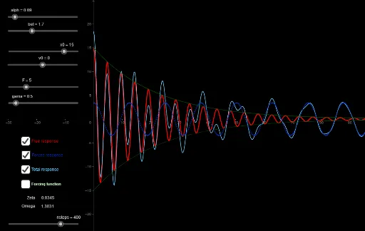
This example demonstrates the dynamic behavior and graphical representation of forced damped oscillations. It involves differential equations, power functions, linear regression, and rhombus geometry, covering concepts like damping vibration, forced vibration, and parameter effects. GeoGebra commands like Sequence, If, and Text are used to construct the model, allowing interactive exploration via sliders. Suitable for high school students and educators studying vibration systems and mathematical modeling.
GeoGebra Commands & Parameters
Sequence(0, 100, 100 / nsteps) → ttIf(x0 ≟ 0, v0 / omega, (sgn(x0) * sqrt(x0^(2) + ((v0 + ((0.5 * x0) * alph)) / omega)^(2)))) → AAIf(x0 ≟ 0, π / 2, atand((v0 + ((0.5 * x0) * alph)) / ((omega * x0)))) → phiText(zet) → text1Text("Zeta") → text2Text(omega) → text3Text("Omega") → text4Sequence(Segment[(tt(i - 1), xxfree(i - 1)), (tt(i), xxfree(i))], i, 2, nsteps) → l1Sequence(Segment[(tt(i - 1), ffforce(i - 1)), (tt(i), ffforce(i))], i, 2, nsteps) → l2Sequence(Segment[(tt(i - 1), xtotal(i - 1)), (tt(i), xtotal(i))], i, 2, nsteps) → l3Sequence(Segment[(tt(i - 1), xforce(i - 1)), (tt(i), xforce(i))], i, 2, nsteps) → l4Sequence(Segment[(tt(i - 1), expoenv(i - 1)), (tt(i), expoenv(i))], i, 2, nsteps) → l5Sequence(Segment[(tt(i - 1), (-expoenv(i - 1))), (tt(i), (-expoenv(i)))], i, 2, nsteps) → l6
AI Drawing Prompt Reference
Create a dynamic graph of forced damped oscillations, including initial position x0, initial velocity v0, damping coefficient alpha, natural frequency omega, and damping ratio zeta. Adjust parameters with sliders to observe the change of displacement x with time t, showing free vibration, forced vibration, total vibration, and the relationship between displacement and time, as well as the attenuation process of damped vibration.
The prompt above was compiled from the original drawing commands and is for reference only.