
Solving a Second-Order ODE Using SolveODE
Loading the math board and drawing, please wait…
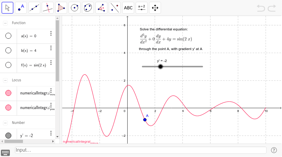
① This GeoGebra example demonstrates the numerical solution of a second-order ordinary differential equation (ODE) using the SolveODE command, showing the solution curve and related numerical integrals. ② Core mathematical concepts include second-order ODEs, numerical solutions, initial value problems, numerical integration, and function graphing. ③ Construction highlights: the SolveODE command is used with objects A, y', a, b, f, and numerical integral results numericalIntegral_minus and numericalIntegral_plus, along with text objects text1, text2, text3 for annotations. ④ Suitable for advanced high school or undergraduate students learning numerical methods for differential equations, and for teachers to demonstrate how parameters affect the solution dynamically.
GeoGebra Commands & Parameters
SolveODE(a, b, f, x(A), y(A), y', -10, 0.1) → numericalIntegral_{minus}SolveODE(a, b, f, x(A), y(A), y', 10, 0.1) → numericalIntegral_{plus}
AI Drawing Prompt Reference
Draw the numerical solution curve of a second-order ordinary differential equation, showing related numerical integral regions in different colors for negative and positive parts, annotate the initial values and the effect of parameters on the solution, presenting the function graph and integral results, suitable for demonstrating dynamic parameter changes in teaching.
The prompt above was compiled from the original drawing commands and is for reference only.