
Exploring Second Order Linear DE with SolveODE
Loading the math board and drawing, please wait…
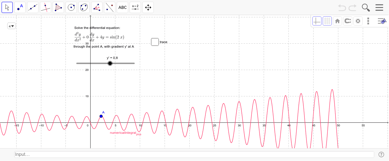
This example demonstrates how to use GeoGebra's SolveODE command to plot solution curves of second-order linear differential equations. Key math concepts include second-order differential equations, solution curves, and linear differential equations. Construction highlights involve commands like Element, SolveODE, SelectedElement, and objects such as flist, Equation, blist, alist, A, a, b, f, y', text1, text2, text3, trace, numericalIntegral_{minus}, c, numericalIntegral_{plus}. Suitable for high school and above students learning numerical solutions and graphical representations of differential equations.
GeoGebra Commands & Parameters
Element(alist, SelectedElement[Equation]) → aElement(blist, SelectedElement[Equation]) → bElement(flist, SelectedElement[Equation]) → fSolveODE(a, b, f, x(A), y(A), y', -20, 0.1) → numericalIntegral_{minus}SelectedElement(Equation) → cSolveODE(a, b, f, x(A), y(A), y', 50, 0.1) → numericalIntegral_{plus}
AI Drawing Prompt Reference
Plot solution curves of a second-order linear differential equation by solving it over two intervals and integrating numerically to visualize the function's behavior, emphasizing the linear properties and shape variations of the solution curves, start by defining the coefficients and function in the equation, then perform numerical integration for two specified intervals, and finally display the results as curves.
The prompt above was compiled from the original drawing commands and is for reference only.