
Projectile Motion with SUVAT Equations and Vectors
Loading the math board and drawing, please wait…
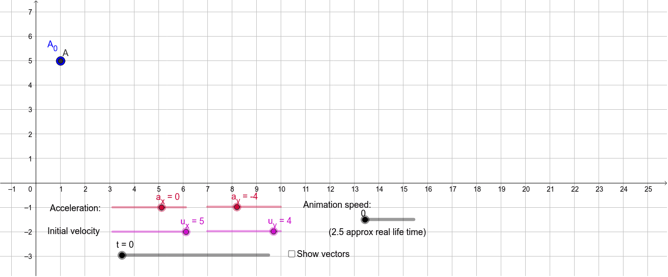
This example demonstrates the trajectory and force analysis of projectile motion. Key math concepts include SUVAT equations, vector operations, and coordinate geometry. Construction highlights involve using commands like Vector for velocity and acceleration vectors, and objects such as u_x, u_y, t, vec_a, A_0, vec_u, vec_v, r_0, vec_s, r, A, arrow_u, arrow_v, arrow_a, arrow_s, animate, text1, text2, text3, a, text4 for dynamic visualization and labeling. Suitable for high school physics and mathematics education to understand the principles of projectile motion and vector applications.
GeoGebra Commands & Parameters
Vector((0, 0), (a_x, a_y)) → vec_aVector((0, 0), (u_x, u_y)) → vec_uVector((0, 0), A_0) → r_0Vector(A_0, A_0 + vec_u) → arrow_uVector(A, A + vec_v) → arrow_vVector(A, A + vec_a) → arrow_aVector(A_0, A_0 + vec_s) → arrow_s
AI Drawing Prompt Reference
Draw a projectile motion trajectory, showing velocity and acceleration vectors. Start from the origin, use arrows to represent the initial velocity and acceleration vectors, and mark the initial position. On the trajectory, indicate the current velocity and acceleration vectors with arrows. Also, use an arrow to show the displacement vector from the initial position to the current position. Suitable for high school physics and mathematics education to understand projectile motion and vector applications.
The prompt above was compiled from the original drawing commands and is for reference only.