
Cartesian and Non-Cartesian Cars
Loading the math board and drawing, please wait…
In collections
MalinC's GeoGebra-book
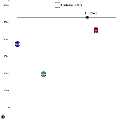
This GeoGebra example illustrates the geometric differences between vehicle motion modeled in Cartesian and non-Cartesian coordinate systems. Key mathematical concepts include function graphs, parametric equations, vector representations, and three-dimensional transformations. Construction utilizes the CurveCartesian command, five function objects (f1–f5), a parameter t, and five points (A1–A5) with coefficients a–e for dynamic control. Suitable for high school analytic geometry and university-level three-dimensional visualization courses.
GeoGebra Commands & Parameters
CurveCartesian(s, f1(s), s, 0, t) → aCurveCartesian(s, f2(s), s, 0, t) → bCurveCartesian(s, f3(s), s, 0, t) → cCurveCartesian(s, f4(s), s, 0, t) → dCurveCartesian(s, f5(s), s, 0, t) → e
AI Drawing Prompt Reference
Draw a graphic showing vehicle motion in Cartesian and non-Cartesian coordinate systems. Include multiple curves representing different vehicle paths, controlled by parameter t. Ensure clear contrast between curves to highlight coordinate system differences. Keep the graphic clear and label key points for understanding.
The prompt above was compiled from the original drawing commands and is for reference only.