
Variations of Cosine Curves
Loading the math board and drawing, please wait…
In collections
Curves
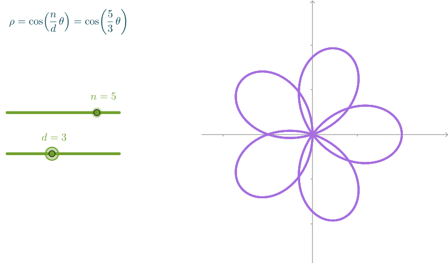
This example demonstrates a family of beautiful polar curves obtained by altering the rational coefficient of the argument in parametric equations. It involves core math concepts like trigonometric functions, polar curves, parametric equations, and graphing. The construction uses GeoGebra commands such as CurveCartesian and Polygon, with objects like sliders (n, d), curves (cur), colors (colRed, etc.), points (A, B, C, D), and text (curText) to illustrate the dynamic changes in the curves. Suitable for high school and above, focusing on parametric equations, polar curves, and function graphing.
GeoGebra Commands & Parameters
CurveCartesian((cos((n / d * θ)); θ), θ, 0, (12 * pi)) → curPolygon(A, B, C, D) → axisHider, a, b, c, d_1
AI Drawing Prompt Reference
Create a family of polar curves demonstrating variations of cosine functions with different parameter values. Generate a parametric polar curve defined by r equals cos of n divided by d times theta, with theta ranging from 0 to 12π. Include two adjustable sliders for parameters n and d to dynamically change the rational coefficient in the curve equation, thereby illustrating how the curve shape transforms. Apply vibrant colors such as red to make the curves stand out clearly. Hide the coordinate axes appropriately to present the curves more elegantly. The visualization should showcase the mathematical relationship between parametric equations and polar curves, demonstrating the diverse forms of trigonometric functions in the polar coordinate system.
The prompt above was compiled from the original drawing commands and is for reference only.