
Demonstration of Space Curve Parameterizations
Loading the math board and drawing, please wait…
In collections
Solution of Systems of nonlinear Equations
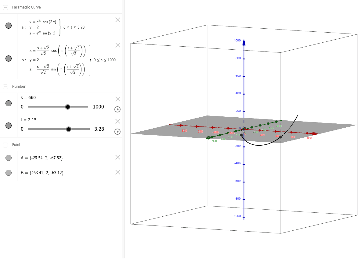
This example illustrates different parameterizations of the same space curve, showcasing the application of parameterization in describing curve motion. Key math concepts include parametric equations, space curves, trigonometric functions, and coordinate geometry. Constructed using GeoGebra's CurveCartesian command with objects like t (parameter), A, b, a, s, B. Suitable for university-level mathematics and engineering students studying space curves and parametric equations.
GeoGebra Commands & Parameters
CurveCartesian(((s + sqrt(2)) / sqrt(2) * cos(log((s + sqrt(2)) / sqrt(2)))), 2, ((s + sqrt(2)) / sqrt(2) * sin(log((s + sqrt(2)) / sqrt(2)))), s, 0, 1000) → bCurveCartesian((ℯ^((2 * t)) * cos((2 * t))), 2, (ℯ^((2 * t)) * sin((2 * t))), t, 0, 3.28) → a
AI Drawing Prompt Reference
Draw a 3D space curve lying in the plane y=2, defined by parametric equations where the x-coordinate is ((s+sqrt(2))/sqrt(2))*cos(ln((s+sqrt(2))/sqrt(2))) and the z-coordinate is ((s+sqrt(2))/sqrt(2))*sin(ln((s+sqrt(2))/sqrt(2))), with parameter s ranging from 0 to 1000. Additionally, draw another space curve also in the plane y=2, with x-coordinate e^(2t)*cos(2t) and z-coordinate e^(2t)*sin(2t), where parameter t ranges from 0 to 3.28. These two curves illustrate different parameterizations of the same underlying space curve, showing their distinct shapes and coverage ranges.
The prompt above was compiled from the original drawing commands and is for reference only.