
Quantitative Frequency Distribution Construction
Loading the math board and drawing, please wait…
In collections
Charts & Graphs
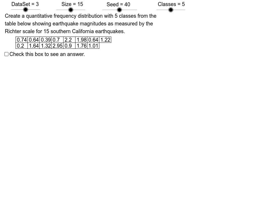
This example demonstrates how to construct quantitative frequency distributions from numerous data samples. It involves core mathematical concepts like data statistics, frequency distribution, histogram, maximum/minimum values, and mean. Key GeoGebra commands and objects used include Sequence, Element, Max, Min, If, KeepIf, Mean, Sort, CountIf, Append, Polygon, Segment, and Sum. Suitable for high school and above students for probability & statistics teaching and data analysis practice.
GeoGebra Commands & Parameters
Sequence(TbTp - k, k, 0, 3) → TbLHSqElement(TbLHSq, 3) → TbLH2Element(RtSq, Mod[Seed, 8] + 1) → RateSequence(Mod[Rate * k + Strt, 20] + 1, k, 0, 19, 1) → OpSqElement(DtSq, Data) → Dt0Sequence(Element[Dt0, Element[OpSq, k]], k, 1, Size) → SmpSqElement(TbLHSq, 1) → TbLH0Element(AcSq, Data) → AcDtMax(SmpSq) → DtMxMin(SmpSq) → DtMnIf(C0 ≤ UB, 0, If[C1 ≤ UB, 0, If[C2 ≤ UB, 1, If[C3 ≤ UB, 2, 3]]]) → AcCWMax(AcDt, AcCW) → AcCnIf(C0 ≤ UB, C0, If[C1 ≤ UB, C1, If[C2 ≤ UB, C2, If[C3 ≤ UB, C3, C4]]]) → ClWdSequence(DtMn + k * ClWd, k, 0, NmCl - 1) → LCLElement(LCL, 2) → LCL2Sequence(UCL1 + ClWd * k, k, 0, NmCl - 1) → UCLSequence(CountIf[Element[LCL, k] ≤ x ≤ Element[UCL, k], SmpSq], k, 1, NmCl) → FrSqMax(FrSq) → FrMxIf(FrMx > 12, 3, If[FrMx > 6, 2, 1]) → VSclElement(TbLHSq, 4) → TbLH3Element(TbLHSq, 2) → TbLH1Element(LCL, 1) → AxMnElement(PlcSq, Data) → DPSequence(k, k, 1, 19) → StrSqKeepIf(floor(20 / x) ≠ 20 / x, StrSq) → RlPrSqSequence(Element[SmpSq, k], k, 1, RwLn1) → DtRw1Sequence(Element[SmpSq, k], k, RwLn1 + 1, Size) → DtRw2Element(DDSq, Data) → DD0Mean(SmpSq) → XbarSort(SmpSq) → SrtSqCountIf(x > 0, RtSq) → RtNoElement(SclSq, Data) → ScaleSequence(If[k > 1, " + ", " "], k, 1, NmCl) → PlsSqSequence(" = ", k, 1, NmCl) → EqSqSequence(DtMn + k * ClWd, k, 0, NmCl - 2) → LCLCn1Append(DtMn, LCLCn1) → LCLCn2Sequence(ClWd, k, 1, NmCl - 1) → CWSq1Append(" ", CWSq1) → CWSq2Sequence(UCL1 + ClWd * k, k, 0, NmCl - 2) → UCLCn1Append(UCL1, UCLCn1) → UCLCn2Sequence("to", k, 1, NmCl) → ToSqSequence(If[Element[FrSq, j] > 0, Sequence["|", k, 1, Element[FrSq, j]], {" "}], j, 1, NmCl) → TlSqPolygon(FDUL, FDLL, FDLR, FDUR) → FDBx, fdrg, fdbt, fdlf, fdtpIf(VScl ≟ 3, ceil(FrMx / 3) * 3, If[VScl ≟ 2, ceil(FrMx / 2) * 2, FrMx]) → VMaxElement(LCL, 1) → LCL1Segment(TbML, TbMR) → tbmdSegment(TbLL, TbLR) → tbbtSegment(TbUL, TbUR) → tbtpSum(FrSq) → ChSzCountIf(x ≠ (0, 0), Dt0) → DtCnSequence(Text[Element[LCL, k], (17.1, CLTp - 0.9 * k)], k, 1, NmCl) → LCLTx1Sequence(Text[Element[EqSq, k], (16.1, CLTp - 0.9 * k)], k, 1, NmCl) → EqTx1Sequence(Text[Element[CWSq1, k], (14.3, CLTp - 0.9 - 0.9 * k)], k, 1, NmCl - 1) → CWTx1Sequence(Text[Element[PlsSq, k], (13.3, CLTp - 0.9 * k)], k, 1, NmCl) → PlsTx1Sequence(Text[Element[LCLCn2, k], (11.6, CLTp - 0.9 * k)], k, 1, NmCl) → LCLCnTxSequence(Text[Element[UCL, k], (26, CLTp - 0.9 * k)], k, 1, NmCl) → UCLTx1Sequence(Text[Element[EqSq, k], (25, CLTp - 0.9 * k)], k, 1, NmCl) → EqTx2Sequence(Text[Element[CWSq1, k], (23.3, CLTp - 0.9 - 0.9 * k)], k, 1, NmCl - 1) → CWTx2Sequence(Text[Element[PlsSq, k], (22.2, CLTp - 0.9 * k)], k, 1, NmCl) → PlsTx2Sequence(Text[Element[UCLCn2, k], (20.5, CLTp - 0.9 * k)], k, 1, NmCl) → UCLCnTxSequence(Segment[(TbLf + CW * k, TbLH0), (TbLf + CW * k, TbLH2)], k, 0, RwLn2) → TbVLnIf(Mod[Size, 2] ≟ 1, Segment[TbMR, TbUR], Segment[TbLR, TbUR]) → tbrgSequence(Text[Element[UCL, k], (15.4, DLHt - 0.9 * k)], k, 1, NmCl) → UCLTx2Sequence(Text[Element[ToSq, k], (14.3, DLHt - 0.9 * k)], k, 1, NmCl) → ToTxSequence(Text[Element[LCL, k], (12.2, DLHt - 0.9 * k)], k, 1, NmCl) → LCLTx2Sequence(Text[Element[FrSq, k], (24.3, DLHt - 0.9 * k)], k, 1, NmCl) → FrTxSequence(If[Element[FrSq, j] > 0, Sequence[Text["|", (17.8 + k * 0.3, DLHt - 0.9 * j)], k, 1, Element[FrSq, j]], Text[" ", (17.8, DLHt - 0.9 * j)]], j, 1, NmCl) → TlTxSqSequence(Text[Element[DtRw1, k], (TbLf - 1.8 + k * CW, TbLH1 + 0.15)], k, 1, RwLn1) → TxRw1Sequence(Text[Element[DtRw2, k], (TbLf - 1.8 + k * CW, TbLH2 + 0.15)], k, 1, RwLn2) → TxRw2If(AcCn ≠ 1, "s", "") → PlCnIf(AcDt ≠ 1, "s", "") → PlDtIf(AcCW ≠ 1, "s", "") → PlCW
AI Drawing Prompt Reference
Create a statistical chart demonstrating the construction of quantitative frequency distributions from multiple data samples. Start by generating a histogram based on the data, marking the maximum and minimum values, and calculating the mean. Then, divide the data into intervals, count the frequency in each, and represent it with bars. Finally, combine all elements into a complete statistical chart, including data points, interval divisions, frequency counts, and the histogram.
The prompt above was compiled from the original drawing commands and is for reference only.