
Central Limit Theorem Demonstration
Loading the math board and drawing, please wait…
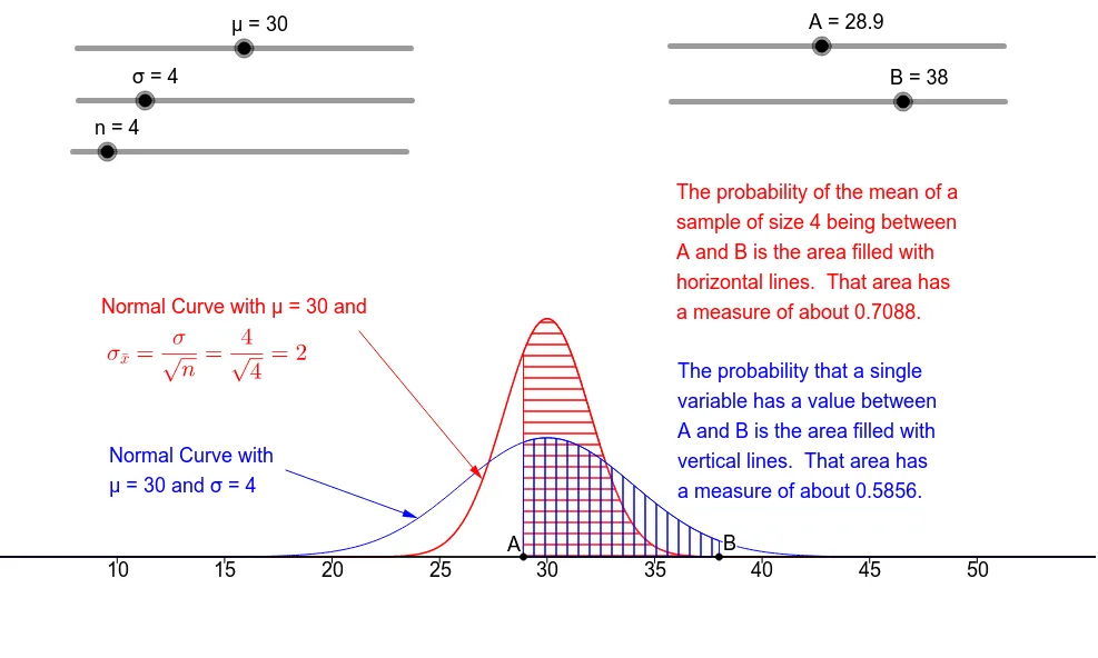
This example visually demonstrates the Central Limit Theorem, showing how the distribution of sample means approaches a normal distribution as the sample size increases. It involves core mathematical concepts like normal distribution, statistics, continuity, logarithm, diagrams, median line, and correlation. The construction utilizes GeoGebra commands such as Sequence, Segment, IntegralBetween, Integral, Polygon, and Vector. Suitable for high school and above students learning advanced statistics.
GeoGebra Commands & Parameters
Sequence(Text[k, (k - 0.5, -0.017)], k, 10, 50, 5) → AxLb2Sequence(Segment[(k, 0), (k, -0.005)], k, 10, 50, 5) → TkSq2Segment((0, 0), (60, 0)) → XAx2IntegralBetween(f, 0, A, B) → M1Integral(g, A, B) → M2Integral((x * f(x)), A, B) → My1Integral((x * g(x)), A, B) → My2Polygon((-5, 0.47), (65, 0.47), (65, 1), (-5, 1)) → ScrnTp, h, i, j, kSegment((0, 0), (60, 0)) → XAx1Vector(E1, D1) → wVector(E2, D2) → a
AI Drawing Prompt Reference
Create a statistical graph demonstrating the central limit theorem. Draw a horizontal axis from 0 to 60 with tick marks and labels at intervals of 5 from 10 to 50. Plot two curves: one representing the original distribution and another for the sample mean distribution, which becomes more normal as sample size increases. Shade the areas under both curves between specified bounds using different colors, and indicate the integral values. Add a semi-transparent rectangle at the top as a title background. From specific points on the curves, draw two arrow vectors pointing to other points to show shifts in mean or variance. Ensure the layout clearly contrasts the distribution shapes and their convergence.
The prompt above was compiled from the original drawing commands and is for reference only.