Sample Size for a Population Mean (Geometric Visualization)

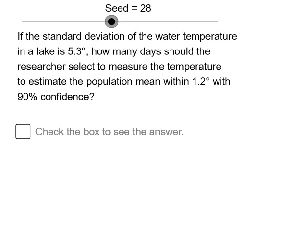
This example demonstrates, via interactive geometric construction, how to determine the required sample size for estimating a population mean given a confidence level and a target margin of error (precision). It focuses on the logic behind confidence intervals: the relation between sampling variability, the confidence factor, the standard error, and the resulting error bound. Core concepts include population-mean estimation, confidence-driven scaling, and the dependence of margin of error on sample size (capturing the inverse/functional relationship). In GeoGebra, the workflow is translated into dynamic objects using Element, Sequence, If, Segment, and CircumcircleArc: Element and Sequence generate and update key computational/graphical entities; If implements conditional choices (e.g., selecting the appropriate confidence-related quantity); Segment provides measurable error/interval lengths; and CircumcircleArc helps visualize confidence-linked curvature/arc measures. Intermediate variables such as squared terms and multiplications (e.g., SDSq, CnfSq, FcSq, MltSq, OESq, Conf, Err) are combined to link statistical calculations with geometric heights and derived measures (e.g., Ht1/Ht2, Sp1/Sp2, Crv1/Crv2). Suitable for high school to early undergraduate probability & statistics, especially for teaching how confidence level and allowable error translate into sample-size requirements using an interactive model.