Practice: Areas Under a Normal Curve

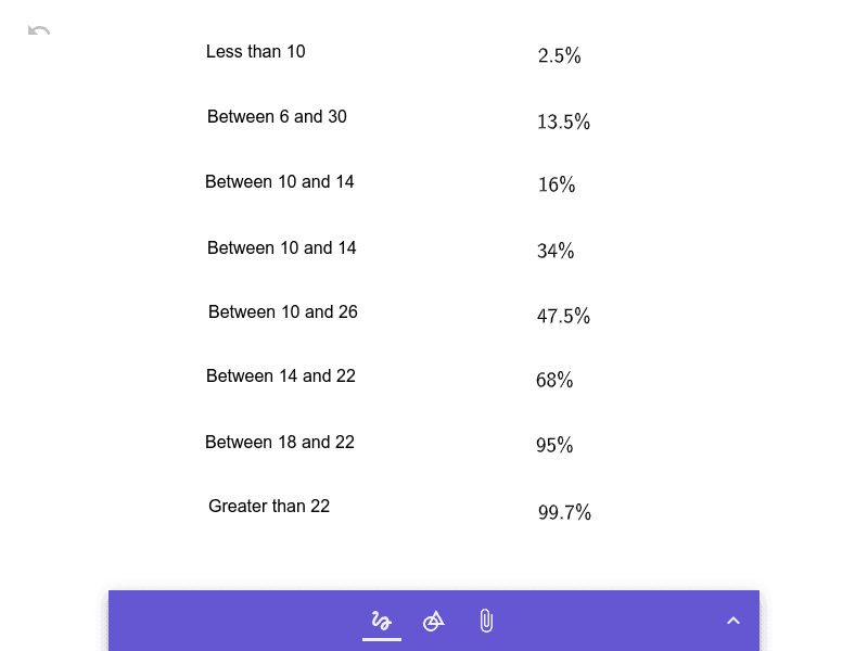
This GeoGebra example visually demonstrates how the area under a normal (Gaussian) curve corresponds to probability for a chosen range of values. It focuses on the probability density function of the normal distribution and the geometric interpretation of area as a quantitative measure. The key ideas include identifying an interval on the x-axis (defining the bounds), plotting the normal curve, and constructing a shaded region bounded by the curve and the interval limits to represent the “area under the curve.” Although no explicit GeoGebra construction commands are provided in the source summary, the model necessarily relies on creating the normal curve (function/curve definition), defining boundary points for the selected range, and using a region/area object to display or compute the enclosed area. Suitable for high school to early university courses in probability & statistics and for calculus-oriented instruction on the connection between integrals and geometric area, especially for students learning to reason from graphs.