
Plotting Real Solutions to Systems of 2 Linear ODEs
Loading the math board and drawing, please wait…
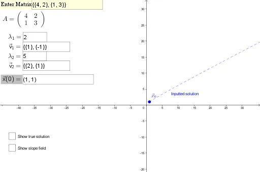
This example demonstrates real solutions to systems of two linear ordinary differential equations (ODEs). Users can input the coefficient matrix and an initial condition to view the exact solution. Key mathematical concepts include differential equations, matrix operations (determinant, inverse matrix), vector fields, and solution trajectories. GeoGebra commands used in construction include Determinant, Identity, SlopeField, SolveODE, and CurveCartesian, making it suitable for university students in mathematics, physics, or engineering to understand the geometric interpretation and numerical solutions of differential equations.
GeoGebra Commands & Parameters
Determinant(A) → detAIdentity(2) → ITextfield(A) → InputBox1Element(A, 1, 1) → aElement(A, 1, 2) → bElement(A, 2, 1) → cElement(A, 2, 2) → dTextfield(x0) → InputBox3CurveCartesian(((c1 * Element[v1(1), 1]) * ℯ^((lambda1 * t))) + ((c2 * Element[v2(1), 1]) * ℯ^((lambda2 * t))), ((c1 * Element[v1(2), 1]) * ℯ^((lambda1 * t))) + ((c2 * Element[v2(2), 1]) * ℯ^((lambda2 * t))), t, 0, 10) → SolnTextfield(lambda1) → InputBox2Textfield(lambda2) → InputBox5Textfield(v1) → InputBox6Textfield(v2) → InputBox7SlopeField(((c * x) + (d * y)) / ((a * x) + (b * y)), 30, 0.5) → slopefield1SolveODE(v(x, y) / u(x, y), x(x0), y(x0), 30, 0.1) → ExactSoln
AI Drawing Prompt Reference
Create a coordinate-plane plot showing both the slope field and solution trajectories for a system of two linear ODEs. Use user-provided parameters: a 2×2 coefficient matrix (four entries) to define the local slope of the direction field, plus initial conditions (x0, y0). Incorporate the given eigenvalue parameters and the corresponding eigenvector component values to form the exact time-dependent expressions for the two state variables. Then render a slope field over the chosen region, and overlay the solution curve(s) that start from (x0, y0), with time ranging roughly from 0 to 10.
The prompt above was compiled from the original drawing commands and is for reference only.