
Slope Fields and Numerical Solutions for First-Order ODEs
Loading the math board and drawing, please wait…
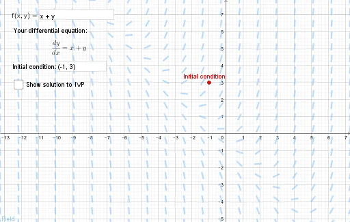
This GeoGebra example demonstrates the slope field (direction field) of a first-order ordinary differential equation dy/dx = f(x,y), allowing users to input the right-hand side function and an initial condition to visualize both the slope field and the corresponding solution curve. Core mathematical concepts include first-order ODEs, the geometric meaning of the derivative as slope, slope fields for qualitative analysis, initial value problems, and numerical approximation methods such as Euler's method. The construction is based on the provided command summary: SolveODE computes precise or numerical solutions; Textfield and InputBox1 enable interactive input of f(x,y) and initial conditions; SlopeField draws the direction field; PointList, PolyLine, EulerList, and Euler construct the Euler polygonal approximation; points A, A1, A2, B1, B2, C1, C2, D1 manage geometric dependencies and visibility; PreciseSoln, NegTimeSoln, showSolution, text1, and text2 control solution display and annotation. This resource is suitable for high school advanced mathematics, university calculus and differential equations courses, and independent learners exploring the qualitative behavior and numerical computation of ODE solutions.
GeoGebra Commands & Parameters
SolveODE(F, x(A), y(A), 100, 0.01) → PreciseSolnTextfield(F) → InputBox1PointList(Transpose[{A1:A100, B1:B100}]) → EulerListPolyLine(EulerList) → EulerSlopeField(F, 20) → FieldSolveODE(F, x(A), y(A), -100, 0.01) → NegTimeSolnTextfield(A) → IC
AI Drawing Prompt Reference
Create a plot combining a slope field and numerical solution paths for a first-order ODE dy/dx = f(x,y). Include an input area for the function f(x,y) and set an initial condition point. Draw the direction (slope) field over a chosen grid scale, so each grid point shows the local tangent slope. Compute and display the solution trajectory passing through the initial point for both positive and negative time directions, and add text that labels the initial condition. Also construct an Euler polygonal approximation as a polyline near the initial point and overlay it with the slope field and the displayed solution curves to illustrate the numerical approximation.
The prompt above was compiled from the original drawing commands and is for reference only.