Plot Complex Solutions of Linear ODE Systems

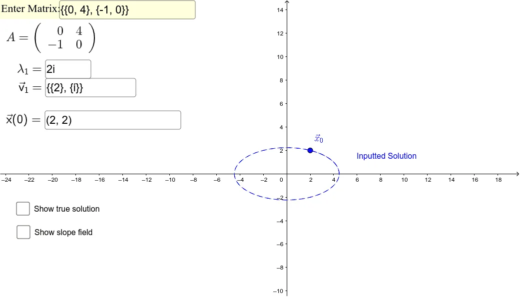
① This GeoGebra example demonstrates how to visualize the true solutions of a system of two linear ordinary differential equations with complex eigenvalues, given a user-input coefficient matrix and initial condition. ② Core mathematical concepts include linear ODE systems, complex eigenvalues, complex exponential solutions, phase-plane trajectories, and decomposition of solutions into real and imaginary parts. ③ Construction highlights: the SolveODE command computes numerical solutions, CurveCartesian plots parametric curves, SlopeField generates a direction field; matrix operations use Determinant, Identity, and Element; interactive inputs via Textfield and InputBox allow adjusting coefficients and initial values; the ComplexSoln object displays the analytic complex-form solution. ④ Suitable for university-level differential equations courses or advanced high-school enrichment, this tool helps learners grasp how complex eigenvalues produce spiral or oscillatory trajectories, and supports classroom demonstrations or self-guided exploration of parameter effects.