
Euler's Method: Numerical Solution of Differential Equations
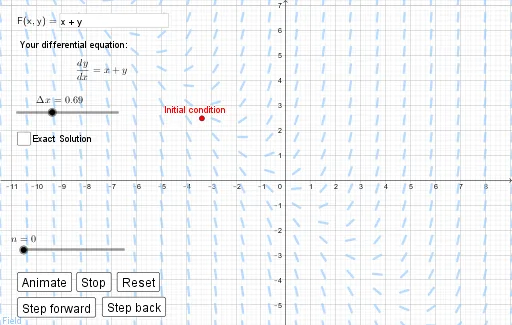
Loading the math board and drawing, please wait…
Euler's Method is a numerical technique for solving differential equations of the form dy/dx = f(x,y) by approximating solutions through iterative steps. Key mathematical concepts include derivatives, function iteration, and numerical computation. Construction involves using SolveODE to input the right-hand side, Textfield for parameters, PointList and PolyLine for plotting points and lines, Sequence and SlopeField to visualize sequences and slope fields. Suitable for high school students or college undergraduates learning calculus fundamentals, useful for mathematical modeling and numerical analysis introductory exercises.
GeoGebra Commands & Parameters
SolveODE(F, x(A), y(A), 100, 0.01) → PreciseSolnTextfield(F) → InputBox1PointList(Transpose[{A1:A100, B1:B100}]) → EulerListPolyLine(EulerList) → EulerSequence(Element[EulerList, i], i, 1, n) → ShownPointsPolyLine(ShownPoints) → NewEulerSlopeField(F, 20) → FieldSequence(Segment[Element[ShownPoints, i] - ((0.4 * step) * (cos(atand(F(Element[ShownPoints, i]))), sin(atand(F(Element[ShownPoints, i]))))), Element[ShownPoints, i] + ((0.4 * step) * (cos(atand(F(Element[ShownPoints, i]))), sin(atand(F(Element[ShownPoints, i])))))], i, 1, n) → EulerSegments
AI Drawing Prompt Reference
Visualize the numerical solution of a differential equation using Euler's method. Start by plotting the exact solution curve, then represent the approximate solution with a sequence of points and a polyline, highlighting some points with a thicker line. Include a slope field to show the direction, and use line segments to indicate the slope at each step, illustrating the geometric meaning of function iteration and numerical computation.
The prompt above was compiled from the original drawing commands and is for reference only.