Demonstrating Taylor Polynomials for Local Approximation

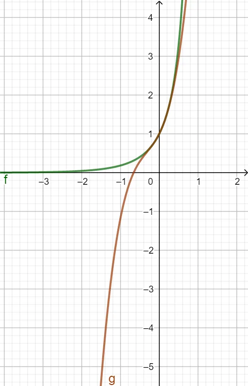
This example demonstrates how to expand a function into a Taylor polynomial to obtain a local approximation around a chosen point, highlighting how the approximation improves as the polynomial order changes. Key concepts include Taylor’s theorem, derivatives evaluated at the expansion point, and the interpretation of functions via power-series-like polynomial approximations. In GeoGebra, you define the target function as an object f (and a comparison object g if used), then construct the Taylor approximation using the command TaylorSeries. The construction relies on the GeoGebra command TaylorSeries applied to the objects f and g, typically allowing the viewer to compare the Taylor polynomial curve/expression with the original function. Suitable for upper-secondary advanced study and early university calculus instruction, especially for teaching the link between derivatives and polynomial approximations.