
Visualization of the Newton-Raphson Method for Root Finding
Loading the math board and drawing, please wait…
In collections
Numerical Methods I - Root Finding
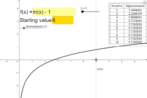
This interactive example demonstrates the iterative process of the Newton-Raphson method to find the roots of a function. It centers on core calculus concepts, specifically the use of derivatives and tangent lines to approximate zeros. The construction utilizes the Tangent command to create linear approximations and the Intersect command to locate the next iteration point on the x-axis. It incorporates InputBox and Textfield for user-defined initial values and TableText to track the convergence of the sequence of approximations. This tool is ideal for high school advanced mathematics or college-level calculus and numerical analysis courses to visualize the convergence behavior of the algorithm.
GeoGebra Commands & Parameters
Textfield(f) → InputBox1OrthogonalLine(Initial, xAxis) → gIntersect(f, g, (6, 0.791759469228055)) → ATangent(A, f) → hIntersect(h, xAxis) → x1OrthogonalLine(x1, xAxis) → iIntersect(f, i, (1.2494431846316703, -0.7773020002238007)) → BTangent(B, f) → jIntersect(j, xAxis) → x2OrthogonalLine(x2, xAxis) → kIntersect(f, k, (2.220637871211863, -0.2022055160122782)) → CTangent(C, f) → lIntersect(l, xAxis) → x3OrthogonalLine(x3, xAxis) → mIntersect(f, m, (2.669663097836665, -0.018047716134800496)) → DTangent(D, f) → n_1Intersect(n_1, xAxis) → x4OrthogonalLine(x4, xAxis) → pIntersect(f, p, (2.717844419601973, -0.0001609266739057702)) → ETangent(E, f) → qIntersect(q, xAxis) → x5TableText({{D1, E1, F1}, {D2, E2, F2}, {D3, E3, F3}, {D4, E4, F4}, {D5, E5, F5}, {D6, E6, F6}, {D7, E7, F7}, {D8, E8, F8}, {D9, E9, F9}, {D10, E10, F10}, {D11, E11, F11}}, "|_ccc") → text1Textfield(setinitial) → InputBox2
AI Drawing Prompt Reference
Draw the graph of function f and use the Newton-Raphson method to find its roots. Start with the initial value input by the user, and construct the iterative process by creating tangents and finding their intersections with the x-axis. Specifically, create a tangent at the initial point, find its intersection with the x-axis, use this intersection point as the new tangent point, and repeat the process until the desired number of iterations is reached. Finally, display the approximate roots for each iteration.
The prompt above was compiled from the original drawing commands and is for reference only.