
Correlation Guess: Estimate ρ from Scatter and Regression Line
Loading the math board and drawing, please wait…
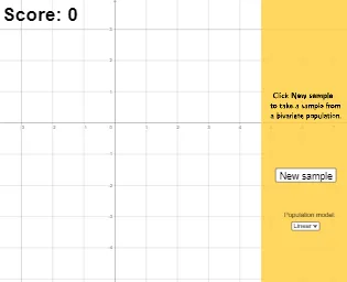
This GeoGebra example demonstrates an interactive workflow where randomly generated scatter points are used to guess the Pearson correlation coefficient ρ, and the guess is then checked against the computed correlation and the corresponding linear regression line. It focuses on core statistics and modeling ideas: Pearson’s correlation (PMCC) to measure linear association, and a least-squares linear fit (FitLineY) to obtain the regression line. Construction highlights include selecting a data model via SelectedIndex, generating sequences and random values with Sequence and RandomUniform, pairing data using Zip, handling logic with If, and computing ρ with PMCC. The visualization layer includes plotting the data set (lists such as xlistNormal/ylistNormal and combined xylist), drawing the regression line (rline), and using Textfield/prompt messages and show/hide flags (e.g., showcorrel, correct/wrong messages) to guide the user through the guessing-and-verification interaction. Suitable for secondary students and early university learners studying probability & statistics, correlation, and regression.
GeoGebra Commands & Parameters
SelectedIndex(models) → chosenmodelSequence(Max[-4, Min[RandomNormal[0, 1], 4]], i, 1, 100) → xlistNormalRandomUniform(1, 3) → bRandomUniform(0.6, 1.5) → aRandomUniform((-sqrt((b + 4) / a)), sqrt((b + 4) / a), 100) → xlistOther, {1.7003313692087823, -1.1277502688964416, -1.4078792452588733, 1.3150959596831446, -0.020381214120730684, 1.6404255909687044, 1.074281299695697, 1.0498008487021717, -1.0627550195170277, -0.7534060318883677, -1.4764562716169511, -1.018908786712169, -0.8005900971521478, 0.6192988627952241, 1.0901308783262877, 1.9084540787821946, 0.9448841059650801, -1.5491789164550809, -1.4444500079819922, 0.12919110819643032, 1.8330270997035567, 1.5778974997993223, -0.2653047203180787, 1.9301898505503894, -1.3177715053332986, -1.7101592944944188, 1.9000943240200023, -1.7365807168324936, -0.34406672994609444, 1.4839370277252233, -1.8184222579683245, 0.45539916210450637, 1.2906079238353498, -0.20606093971558503, -1.659444940315778, -0.4609767523820443, -0.3265096233838727, -0.0651585713579168, 0.34719700184103774, 0.8892401836490491, 1.735200632763472, 1.2477686229659948, 1.2613627022567548, -0.2680196214179382, -0.2335013050632253, 0.4923454768926929, -0.20283920019997081, -0.4424142235270745, 1.3863952222126603, -0.6402037848894637, -0.19065385600626494, -0.22461193683024683, -0.08477931779156744, -1.50058964269489, -1.7316215344420485, -0.45341502298914604, 1.8020659143819382, -0.13966839665367337, -1.6047262767437025, 1.4554501567766442, 1.049189221303305, 1.5179787775945914, 0.22851482307218274, -0.5177805397564215, -1.0972734216267188, 1.5059566301744465, 1.8606390712853715, 0.6247416428711541, -0.3441529735573894, -0.3727403137179077, -0.27649149007175566, -1.2854324369032597, -0.027879960513713664, 1.1048201242788573, -1.5250223569924324, 0.2102316896005194, -0.9274448332524461, 0.598311295531958, 0.362893748897126, -1.6180266935823004, -1.688771307783909, 1.2519088633190194, 1.7846433048997674, -0.6318082096428963, 0.33283235704586134, 1.9224252131911943, 0.07303951759284177, -1.5065088483508118, -1.2086549795974193, -0.4884796012488888, 0.7824516894745781, -1.2252411026153256, -0.6048734379826703, 0.9336299739928646, -0.8206653662604222, 0.023618947536423907, -0.38462832127061675, 1.741603331636153, -0.537689389470976, 0.05141142380062402}If(chosenmodel ≟ 1, xlistNormal, xlistOther) → xlistRandomUniform(-1, 1) → rhoZip(Max[-4, Min[(rho * xx) + (sqrt(1 - rho^(2)) * RandomNormal[0, 1]), 4]], xx, xlist) → ylistNormalZip(Max[-4, Min[f(xx) + RandomNormal[0, c], 4]], xx, xlist) → ylistOtherIf(chosenmodel ≟ 1, ylistNormal, ylistOther) → ylistZip((xx, yy), xx, xlist, yy, ylist) → xylistPMCC(xylist) → rFitLineY(xylist) → rlinePolygon(Corner[2], Corner[3], (0.75 * Corner[3]) + (0.25 * Corner[4]), (0.75 * Corner[2]) + (0.25 * Corner[1])) → panel, g, h, i, jIf(abs(guess - r) > 0.2, 0, If[0.1 < abs(guess - r) ≤ 0.2, 1, If[abs(guess - r) ≤ 0.1, 2, 3]]) → guessstateTextfield(guessinput) → InputBox1
AI Drawing Prompt Reference
Create a set of random scatter plots with normally distributed and non-normally distributed data points. Calculate the Pearson correlation coefficient for the scatter plot and draw the regression line based on the coefficient. The user needs to estimate the correlation coefficient from the graph and compare it with the calculated coefficient; correct estimation will show a correct message.
The prompt above was compiled from the original drawing commands and is for reference only.