
Interactive Introduction to the Correlation Coefficient with Data and Line Fitti
Loading the math board and drawing, please wait…
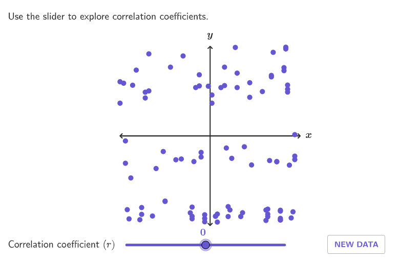
This GeoGebra example visualizes how two data sets correspond to the correlation coefficient by dynamically generating scatter data and comparing it with a reference/fit line. Learners can interpret what the correlation coefficient means as the observed linear trend changes, including the direction implied by the slope. The core math concepts are the (Pearson) correlation coefficient (PMCC), linear relationship versus correlation-not-causation, and how line slope/linear fit relates to the strength and direction of association. Construction highlights include using Shuffle, Sequence, Sample, and KeepIf to generate and filter points/data; employing Line/Segment/Polygon for reference geometry; using Element/Translate/Corner to map and place elements in the coordinate system; using Slope to extract trend direction; adding Text/labels for prompts and computed values; and computing the correlation via PMCC while guiding the interaction with sliders and guideline objects (e.g., horizontal/vertical guides) for dynamic exploration. Suitable for grades 9–12 probability & statistics, especially model-based prediction and interpreting correlation in classroom discussions or inquiry tasks.
GeoGebra Commands & Parameters
Shuffle(Sequence[-4, -1, 0.2]) → v1s, {-2.8, -3.5999999999999996, -2.5999999999999996, -4, -2, -1.2000000000000002, -1.6, -1, -1.8, -3, -3.1999999999999993, -1.4000000000000001, -3.3999999999999995, -2.1999999999999993, -3.8, -2.3999999999999995}Shuffle(Sequence[0, 4, 0.2]) → v2s, {0.4, 2.2, 3.6000000000000005, 3, 3.8000000000000007, 1.2, 1.7999999999999998, 1.5999999999999999, 1, 0.6000000000000001, 2.8000000000000007, 3.4000000000000004, 3.2, 0, 0.2, 0.8, 4, 2.4000000000000004, 1.4, 2, 2.6000000000000005}Shuffle({1 / 10, 1 / 5, 1 / 3, 1 / 2, 1, 3, 4, 5, 9, 10}) → frequencies, {3, 0.2, 0.5, 4, 10, 0.3333333333333333, 5, 0.1, 9, 1}Corner(5) → AppSizeElement(v1s, Mod[example, Length[v1s]] + 1) → v1Element(v2s, Mod[example, Length[v2s]] + 1) → v2Line((-5, v1), (5, v2)) → gSlope(g) → slpSequence(RandomNormal[0, (((1 - r^(2)) * (r^(2) + 0.1)) * 5)], ii, 1, 100) → l2, {-0.24865600393024015, -0.4427163928876197, -0.06436210133034098, -0.7246319666843015, 0.1518131634784586, 0.2783136548947105, -0.08877464593912159, -0.24058088448183162, -0.05712717781762687, -0.06423043757026925, 0.39825486588386466, 0.7075312066655958, -0.3262376427966622, -0.5723245120750319, -0.27928180563388555, -0.07049671607224141, 0.11852623574981205, -0.1463807178102759, 0.32525153572259174, -0.1842690692292607, -0.4747902410008965, 0.0832416549280435, 0.5311078737767596, 0.19730645485737308, -0.1296478081407259, 0.18735619858140565, 0.31400317616087886, -0.12257898186089448, 0.6087135165018176, -1.279155909882137, 0.2827494470950619, -0.23100518632541264, -0.08981478843637765, -0.9689171778513928, 0.23848140358592615, 1.0245434582157533, -0.6040482362219812, 0.7308526648335587, -0.2128144312592865, 0.23769152491819634, 0.9317973687320863, -0.7499051450311507, -0.04395514429968953, 0.5825030431754739, -0.9129946765796846, 0.13420294834548918, 0.0964497163074819, -0.32540220629108846, -0.27157799250002157, -0.7984497778844687, 0.08825112557947422, 1.1558360033689312, -0.2746119731854489, 0.5162099281346505, -0.3332501829911684, -0.3812971389014234, 0.15746428357187267, 0.11959749773574901, 0.01122581881267802, -0.39624077657157447, -0.3585295005697764, -0.8226532437499681, -0.7656341447433536, 0.12230599920670075, 0.1320565815170991, -0.40488749810086977, 0.13333504974605417, -0.6523812111577524, 0.5031527678652897, 0.08227681019297829, -0.3407671265640928, 0.30434097036692154, 0.06790200065394335, -0.33507998440307635, -0.43360831610784045, 0.627308460110241, 0.002199833979304936, 0.06352829010100344, 0.5439244093003046, -0.3204633620044284, -0.6497569867185523, 0.24045007334481863, -0.31569812366433053, 0.12094517804052977, 1.4901306986156224, 0.08139998093222266, -0.011035814245865114, 0.14073615260172131, 0.7974913927879635, -0.047794937202976014, 0.05481483990259745, 0.03779061937276644, 0.6867733019435083, -0.41580916304592114, 0.11181834570481163, -0.11922560710612219, 0.1317711898668424, -0.021782237243583923, 0.033727151690141906, -0.3620900224723636}Sample(Sequence[-5, 5, 0.1], 100, true) → l1, {4.299999999999999, -1.9, -2.5999999999999996, -4.400000000000002, -1.0999999999999992, -4.700000000000001, 4.299999999999999, 2.3000000000000003, 1.4000000000000004, 3.1, -5, -2.4999999999999996, -3.5999999999999996, 4.6999999999999975, 1.2000000000000002, -1, -0.30000000000000016, -3.1999999999999993, 4.1, 3.2, 0.6, 3.900000000000001, 1.5000000000000004, 4.199999999999999, 3.4000000000000004, -4.100000000000003, 1.1, -0.5000000000000001, 1, 0.1, 1.9000000000000008, 0.7999999999999999, -0.30000000000000016, -4.700000000000001, -1.3999999999999995, -2.8, -4.800000000000001, -2.4999999999999996, -0.9, 3.2, -2.1999999999999993, 2.2, 3.2, -1, -3.3999999999999995, -0.5000000000000001, 3.7000000000000006, 0.4, -0.30000000000000016, -5, 1.7000000000000006, -3.3999999999999995, 1.5000000000000004, 3.1, -0.10000000000000014, -0.6000000000000001, 4.1, 1.8000000000000007, -1.5999999999999996, -3.9, -3, 0.1, 4.6999999999999975, -4.600000000000001, 4.499999999999998, 3.900000000000001, 3.900000000000001, 3.3000000000000003, 4.899999999999997, 4.199999999999999, -0.8, -3.8, -1, -4.500000000000002, 3.8000000000000007, 4.6999999999999975, 4.599999999999998, 2.2, 0.8999999999999999, 3.900000000000001, -3.5999999999999996, -0.6000000000000001, 3.5000000000000004, 0.4, -1.4999999999999996, -4.500000000000002, 4.399999999999999, 4.299999999999999, 0.7999999999999999, 3.4000000000000004, 1, 0.30000000000000004, -3.8, 3.900000000000001, 3.7000000000000006, 4.199999999999999, -4.3000000000000025, 4.199999999999999, 0.30000000000000004, 2.900000000000001}Element(frequencies, Mod[example, Length[frequencies]] + 1) → frecTranslate(vGuideline, Vector[(Vector[Corner[1], Corner[2]] / 800 * 16)]) → vGuideline'Polygon({ViewCorner1_{1}, (x(ViewCorner3_{1}), y(ViewCorner1_{1})), ViewCorner3_{1}, (x(ViewCorner1_{1}), y(ViewCorner3_{1}))}) → q1_{1}Segment((x(ViewCorner1_{1}), 0), (x(ViewCorner3_{1}), 0)) → xAxisFake_{1}Segment((0, y(ViewCorner1_{1})), (0, x(ViewCorner3_{1}))) → yAxisFake_{1}Text("x", (x(ViewCorner3_{1}), 0.1), true, true, 1, 0) → text1_{1}Text("y", (0, y(ViewCorner3_{1})), true, true, 0, 1) → text2_{1}Translate(hGuideline, Vector[(Vector[Corner[1], Corner[4]] / 500 * 16)]) → hGuideline'Zip((xx, (r * f(xx)) + (h1(xx) * (1 - abs(r))) + ii), xx, l1, ii, l2) → l3KeepIf(abs(y(PP)) ≤ 5, PP, l3) → l4PMCC(l4) → a
AI Drawing Prompt Reference
This is an interactive graph showing scatter plots and a fitted line for two datasets. Users can dynamically adjust data points to observe changes in the correlation coefficient. The graph includes scatter data, a fitted line, slope, correlation coefficient calculation results, and labels. Construction order: first generate points for both datasets, then draw the fitted line, calculate slope, generate random data points and fit, and finally add labels and axes.
The prompt above was compiled from the original drawing commands and is for reference only.