
Phase Plane by Pablo Rodríguez-Sánchez
Loading the math board and drawing, please wait…
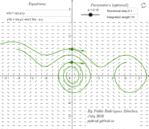
This example demonstrates the concept of a phase plane, involving solutions to differential equations. Using GeoGebra commands like SlopeField and Vector, phase trajectories can be visually displayed. Suitable for calculus and ordinary differential equations courses.
GeoGebra Commands & Parameters
SlopeField(v(x, y) / u(x, y), N, l, xmin, ymin, xmax, ymax) → slopefield1Textfield(u) → InputBox1Textfield(v) → InputBox2SolveODE(v(x, y) / u(x, y), x(A), y(A), tmin, numStep) → fAbackSolveODE(v(x, y) / u(x, y), x(A), y(A), tmax, numStep) → fAforwSolveODE(v(x, y) / u(x, y), x(B), y(B), tmin, numStep) → fBbackSolveODE(v(x, y) / u(x, y), x(B), y(B), tmax, numStep) → fBforwVector((u(x(B), y(B)), v(x(B), y(B)))) → VBUnitVector(VA) → vAUnitVector(VB) → vBVector(A, A + vA) → v_AVector(B, B + vB) → v_BImplicitCurve(u(x, y)) → IsoclineXImplicitCurve(v(x, y)) → IsoclineYTextfield(numStep) → InputBox3Textfield(tmax) → InputBox4
AI Drawing Prompt Reference
Draw a phase plane for differential equations, including a direction field and trajectories. Start by plotting the direction field represented by the ratio of two functions, then trace forward and backward from initial points to show trajectories, add unit vectors extending from these points, and finally include isoclines to illustrate slope relationships.
The prompt above was compiled from the original drawing commands and is for reference only.