
Change of Basis by Pablo Rodríguez-Sánchez
Loading the math board and drawing, please wait…
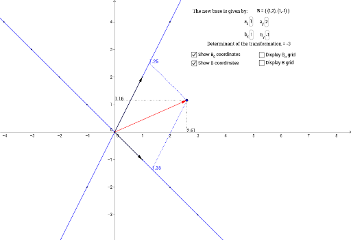
This example illustrates the concept of change of basis in linear algebra. By inputting vectors and bases, it visually demonstrates how vectors are represented differently under various bases. Commands like Vector, Segment, Line, and Intersect are used, suitable for linear algebra courses.
GeoGebra Commands & Parameters
Textfield(a_x) → inputBox1Textfield(a_y) → inputBox2Textfield(b_x) → inputBox3Textfield(b_y) → inputBox4Vector((a_x, a_y)) → aVector((b_x, b_y)) → bVector(R) → rSegment(R, (x(R), 0)) → SegmentXBcSegment(R, (0, y(R))) → SegmentYBcLine((0, 0), a) → AxisXBLine((0, 0), b) → AxisYBLine(R, a) → LineXBLine(R, b) → LineYBIntersect(AxisXB, LineYB) → AuxXBIntersect(AxisYB, LineXB) → AuxYBSegment(AuxXB, R) → SegmentXBSegment(AuxYB, R) → SegmentYBDeterminant(MatrixBtoBc) → detInvert(MatrixBtoBc) → MatrixBctoBSequence(Line[(t, 0), (t, 1)], t, (-TicksMax), TicksMax, 1) → GridXBcSequence(Line[(0, t), (1, t)], t, (-TicksMax), TicksMax, 1) → GridYBcSequence(Point[(0, 0), Vector[(a * t)]], t, (-TicksMax), TicksMax, 1) → TickMarksXBSequence(Point[(0, 0), Vector[(b * t)]], t, (-TicksMax), TicksMax, 1) → TickMarksYBSequence(Line[Point[(0, 0), Vector[(a * t)]], b], t, (-TicksMax), TicksMax, 1) → GridXBSequence(Line[Point[(0, 0), Vector[(b * t)]], a], t, (-TicksMax), TicksMax, 1) → GridYB
AI Drawing Prompt Reference
Draw two basis vectors in a coordinate system and visualize how the same vector is represented differently under various bases. Start by plotting the axes defined by the basis vectors, then show the transformation of a vector's coordinates under different bases. Include grid lines and tick marks to clearly illustrate the differences in representation, suitable for linear algebra education.
The prompt above was compiled from the original drawing commands and is for reference only.