
Interactive Truncated Fourier Series
Loading the math board and drawing, please wait…
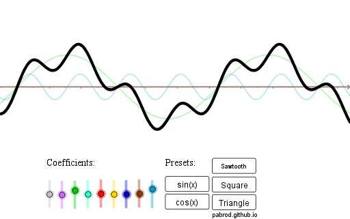
This example demonstrates the graphical behavior of a truncated Fourier series through an interactive interface. It involves core mathematical concepts such as Fourier series, trigonometric functions, and function approximation. The construction leverages GeoGebra commands/objects like b_1, b_2, b_3, s_3, s_2, s_1, a_3, c_3, a_1, c_1, a_2, c_2, button1, button2, a_0, c_0, b_4, s_4, a_4, c_4, f, button3, button4, button5, text1, text1_1, text2. It is suitable for university students in mathematics or physics, and enthusiasts interested in Fourier series.
GeoGebra Commands & Parameters
100s_3(x) = (b_3 * sin((3 * x)))s_2(x) = (b_2 * sin((2 * x)))s_1(x) = (b_1 * sin(x))0c_3(x) = (a_3 * cos((3 * x)))0c_1(x) = (a_1 * cos(x))0c_2(x) = (a_2 * cos((2 * x)))Numeric a_0(0.0)c_0(x) = a_0 / 2Numeric b_4(0.4)s_4(x) = (b_4 * sin((4 * x)))0c_4(x) = (a_4 * cos((4 * x)))f(x) = c_0(x) + c_1(x) + c_2(x) + c_3(x) + c_4(x) + s_1(x) + s_2(x) + s_3(x) + s_4(x)
AI Drawing Prompt Reference
Create an interactive graphical representation of a truncated Fourier series, demonstrating the behavior of Fourier series. Include basic sine and cosine functions, and their combinations, from the lowest to the fourth order, showing the function approximation effect. Start with a pure zero function, gradually adding sine and cosine terms of each order via buttons to eventually form the target function graph.
The prompt above was compiled from the original drawing commands and is for reference only.