
First Order Linear Differential Equation
Loading the math board and drawing, please wait…
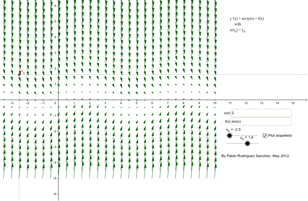
This example demonstrates solving a first order linear differential equation with a given initial condition and plotting its slope field. Key mathematical concepts include first order linear differential equations and slope fields. It utilizes commands like Integral, Textfield, Line, Intersect, Sequence in GeoGebra. Suitable for calculus courses.
GeoGebra Commands & Parameters
Integral(u) → Int_1Textfield(u) → inputBox1Textfield(f) → inputBox2Integral((f(x) * ℯ^(Int_1(x) - Int_1(x_0)))) → Int_2Line((x_0, 0), (x_0, 1)) → LineXLine((0, y_0), (1, y_0)) → LineYIntersect(LineX, LineY) → P_0Sequence(Sequence[Vector[(i / 2, j / 2), (i / 2 + d, j / 2 + (d * (f(i / 2) - (j / 2 * u(i / 2)))))], j, -10, 20], i, -10, 20) → Slopefield
AI Drawing Prompt Reference
Draw a slope field for a first-order linear differential equation. Start by placing two input boxes on the coordinate plane for entering the function and coefficient. Then draw two reference lines: a vertical dashed line through the x-coordinate of the initial point and a horizontal dashed line through the y-coordinate, with their intersection marked as the initial point. Next, compute and plot the particular solution curve that passes through this initial point, smoothly traversing the slope field. Finally, fill the grid with short line segments at regular intervals, each indicating the slope direction at that point, to form the complete slope field. The overall graph should clearly show the relationship between the slope field and the solution curve.
The prompt above was compiled from the original drawing commands and is for reference only.