
Population Exponential Growth Slope Field- First Order Differential Equations
Loading the math board and drawing, please wait…
In collections
Differential equation Material
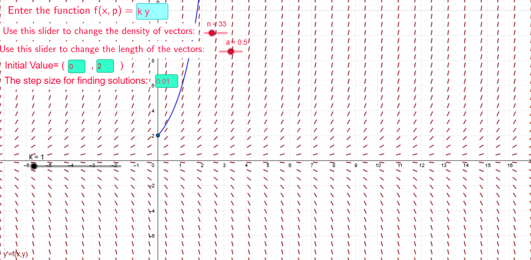
This example demonstrates the slope field of a population exponential growth model, visually representing the distribution of solution curves for first-order differential equations. Key mathematical concepts include first-order differential equations, exponential growth models, slope fields, and solution curves. It is constructed using GeoGebra commands like Textfield, SlopeField, SolveODE, and objects such as k, f, InputBox1, n, a, slopefield1, text1, etc. Suitable for high school students and beginners in differential equations.
GeoGebra Commands & Parameters
Textfield(f) → InputBox1SlopeField(f, n, a) → slopefield1Textfield(a) → InputBox2Textfield(c) → InputBox3Textfield(d) → InputBox4SolveODE(f, c, d, 5, b) → numericalIntegral1Textfield(b) → InputBox5
AI Drawing Prompt Reference
Create a slope field diagram for a first-order differential equation modeling exponential population growth. Include an input box for the differential equation expression, a slope field composed of small line segments whose directions and lengths indicate the slope of solution curves at each point, and three additional input boxes for setting the initial independent variable value, the initial dependent variable value, and a parameter for the endpoint of the solution curve. Display one approximate solution curve obtained numerically, starting from the specified initial point and following the slope field direction. The diagram should illustrate how solution curves vary with different initial conditions, showing exponential growth behavior.
The prompt above was compiled from the original drawing commands and is for reference only.