
Slope Field and Numerical Integration of a Differential Equation
Loading the math board and drawing, please wait…
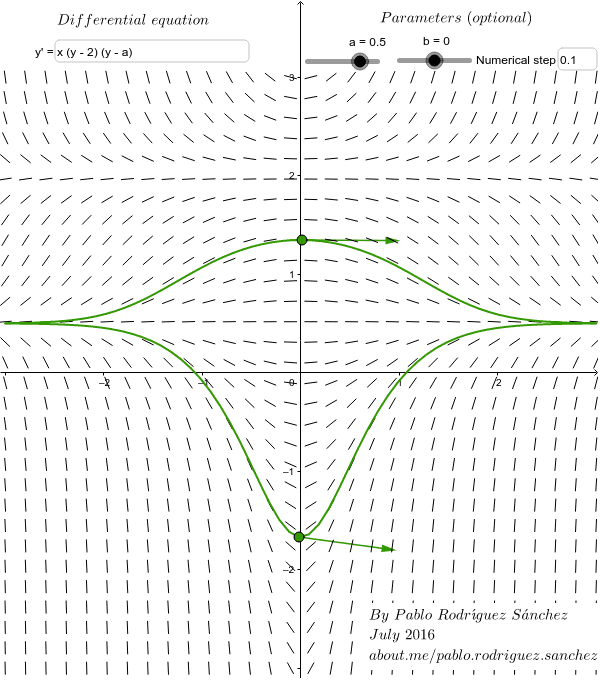
This example demonstrates the slope field and numerical integration of a differential equation. It involves key concepts in calculus such as slope fields and numerical integration methods. Using GeoGebra commands like SlopeField and SolveODE, it provides a visual understanding of differential equation solutions. Suitable for high school math education, particularly calculus courses.
GeoGebra Commands & Parameters
SlopeField(v(x, y) / u(x, y), N, l, xmin, ymin, xmax, ymax) → slopefield1Textfield(u) → InputBox1Textfield(v) → InputBox2SolveODE(v(x, y) / u(x, y), x(A), y(A), tmin, numStep) → fAbackSolveODE(v(x, y) / u(x, y), x(A), y(A), tmax, numStep) → fAforwSolveODE(v(x, y) / u(x, y), x(B), y(B), tmin, numStep) → fBbackSolveODE(v(x, y) / u(x, y), x(B), y(B), tmax, numStep) → fBforwVector((u(x(B), y(B)), v(x(B), y(B)))) → VBUnitVector(VA) → vAUnitVector(VB) → vBVector(A, A + vA) → v_AVector(B, B + vB) → v_BImplicitCurve(u(x, y)) → IsoclineXImplicitCurve(v(x, y)) → IsoclineYTextfield(numStep) → InputBox3
AI Drawing Prompt Reference
Draw a slope field for a differential equation, with a grid of short line segments covering the plot area. From two starting points, extend four solution curves, two forward and two backward, each following the slope field smoothly. At each starting point, draw a unit direction vector indicating the tangent direction. Also plot two isoclines corresponding to the zero curves of the numerator and denominator functions, intersecting the slope field. Include three input boxes for adjusting the two component functions and the numerical integration step size.
The prompt above was compiled from the original drawing commands and is for reference only.