
Dot Plot Analysis
Loading the math board and drawing, please wait…
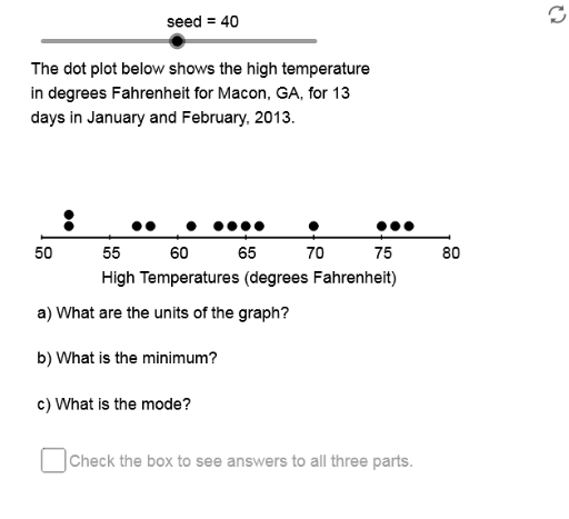
This example demonstrates how to analyze data distribution using dot plots, covering core math concepts like statistical analysis, central tendency (mean, median, mode), and data spread. It utilizes GeoGebra commands and objects such as Mod, Element, Sequence, Max, Min, Sort, Length, Segment, Median, mean, If, along with elements like RPSq, seed, PrmFct for constructing the plot. Suitable for high school mathematics education, focusing on probability & statistics and data processing skills.
GeoGebra Commands & Parameters
Mod((seed * PrmFct), Cmpst) → Nmbr1Element(DSSq, Chc0) → DS0Element(RPSq, Chc4) → RateSequence(Element[DS0, Mod[Strt + (Rate * k), 20] + 1], k, 1, SmpSz) → SmpMax(Smp) → SmpMxMin(Smp) → SmpMnMax(Acc, If[(5 * AxLB) ≤ AxUB, (5 * AxLB), If[(2 * AxLB) ≤ AxUB, (2 * AxLB), AxLB]]) → AxSclSequence(k, k, SmpMn, SmpMx, Acc) → SmpDmnSequence(Element[Smp, k], k, 1, RN1) → SmpRw1Sort(Intersection[SmpDmn, Smp]) → SmpVlsLength(SmpVls) → RngCntSequence(CountIf[x ≟ Element[SmpVls, k], Smp], k, 1, RngCnt) → FrqSqSegment(LE, RE) → haxSequence(Element[Smp, k], k, RN1 + 1, SmpSz) → SmpRw2Sequence(Sequence[(Adp(Element[SmpVls, k]), GrHt + (0.05 * j)), j, 1, Element[FrqSq, k]], k, 1, RngCnt) → DotsSequence(k, k, AxMn, AxMx, AxScl) → LbSqSequence(Segment[(GrLf + (k * SF), GrHt - 0.01), (GrLf + (k * SF), GrHt + 0.01)], k, 0, AxRng, AxScl) → AxTcElement(DDSq, Chc0) → DD0Sequence(Text[k, (Adp(k) - 0.9, GrHt - 0.09)], k, AxMn, AxMx, AxScl) → LbSqTxElement(AxLbSq, Chc0) → AxTtlLength(LbSq) → LblCntLength(DS0) → DtStSzMedian(Smp) → SmpMdnmean(Smp) → SmpAvgIf(SmpAvg < SmpMdn, "skewed left", If[SmpAvg > SmpMdn, "skewed right", "symmetric"]) → SmpSkwIf(Chc1 ≟ 1, "minimum", "maximum") → MxOMnMode(Smp) → SmpMod0If(Min[FrqSq] ≟ Max[FrqSq], {}, SmpMod0) → SmpMod1Element(UntSq, Chc0) → UntIf(Chc1 ≟ 1, SmpMn, SmpMx) → AnsBNmbr
AI Drawing Prompt Reference
Create a dot plot analysis chart showing the distribution of a dataset. The horizontal axis represents numerical values with tick marks and labels, while the vertical axis indicates frequency. Each data point is a small dot, with identical values stacked vertically. Include a horizontal axis line, and display the mean, median, and mode as reference lines or labels. Annotate the skewness (left, right, or symmetric) based on the data. Also mark the minimum and maximum values. The chart should be clean and suitable for high school statistics education.
The prompt above was compiled from the original drawing commands and is for reference only.