
Visualizing the Normal Distribution: PDF and CDF
Loading the math board and drawing, please wait…
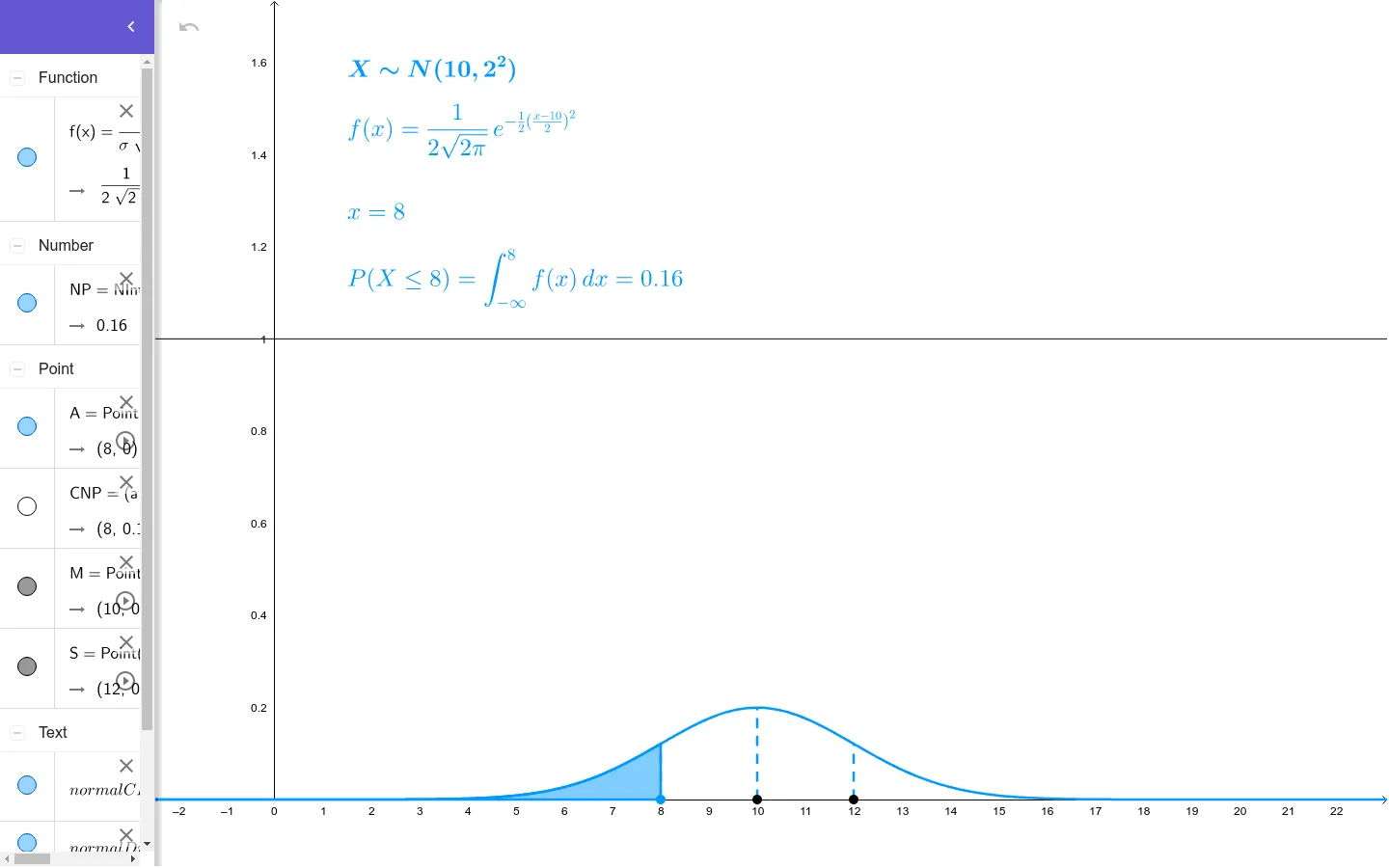
① This GeoGebra example dynamically illustrates the normal distribution's probability density function (bell curve) and its cumulative distribution function, showing how the mean μ and standard deviation σ shape the curve. ② Core mathematical concepts include the normal distribution, probability density function (PDF), cumulative distribution function (CDF), mean, standard deviation, and the use of integrals in probability calculations. ③ Construction highlights: Point creates key points (e.g., mean M, standard deviation σ), NIntegral computes cumulative probabilities, Segment draws auxiliary lines, and objects like normalDistribution, normalPDF, and normalCDF build the visual, with sliders (a, b) for dynamic interval adjustment. ④ Suitable for high school to college-level probability and statistics courses, as well as AP Statistics or calculus, helping learners intuitively explore properties of continuous random variables and the connection to integration.
GeoGebra Commands & Parameters
Point(xAxis) → MPoint(xAxis) → APoint(xAxis) → SNIntegral(f, μ - (10 * σ), a) → NPSegment((μ, 0), (μ, f(μ))) → hSegment((μ + σ, 0), (μ + σ, f(μ + σ))) → iSegment((μ - σ, 0), (μ - σ, f(μ - σ))) → j
AI Drawing Prompt Reference
Draw the probability density function (PDF) and cumulative distribution function (CDF) of the normal distribution. Start by creating three points on the x-axis to represent the mean μ and standard deviation σ, then use integration to compute cumulative probabilities, and finally draw auxiliary lines to show the positions of the mean and standard deviation.
The prompt above was compiled from the original drawing commands and is for reference only.