
Binomial vs. Normal Distribution
Loading the math board and drawing, please wait…
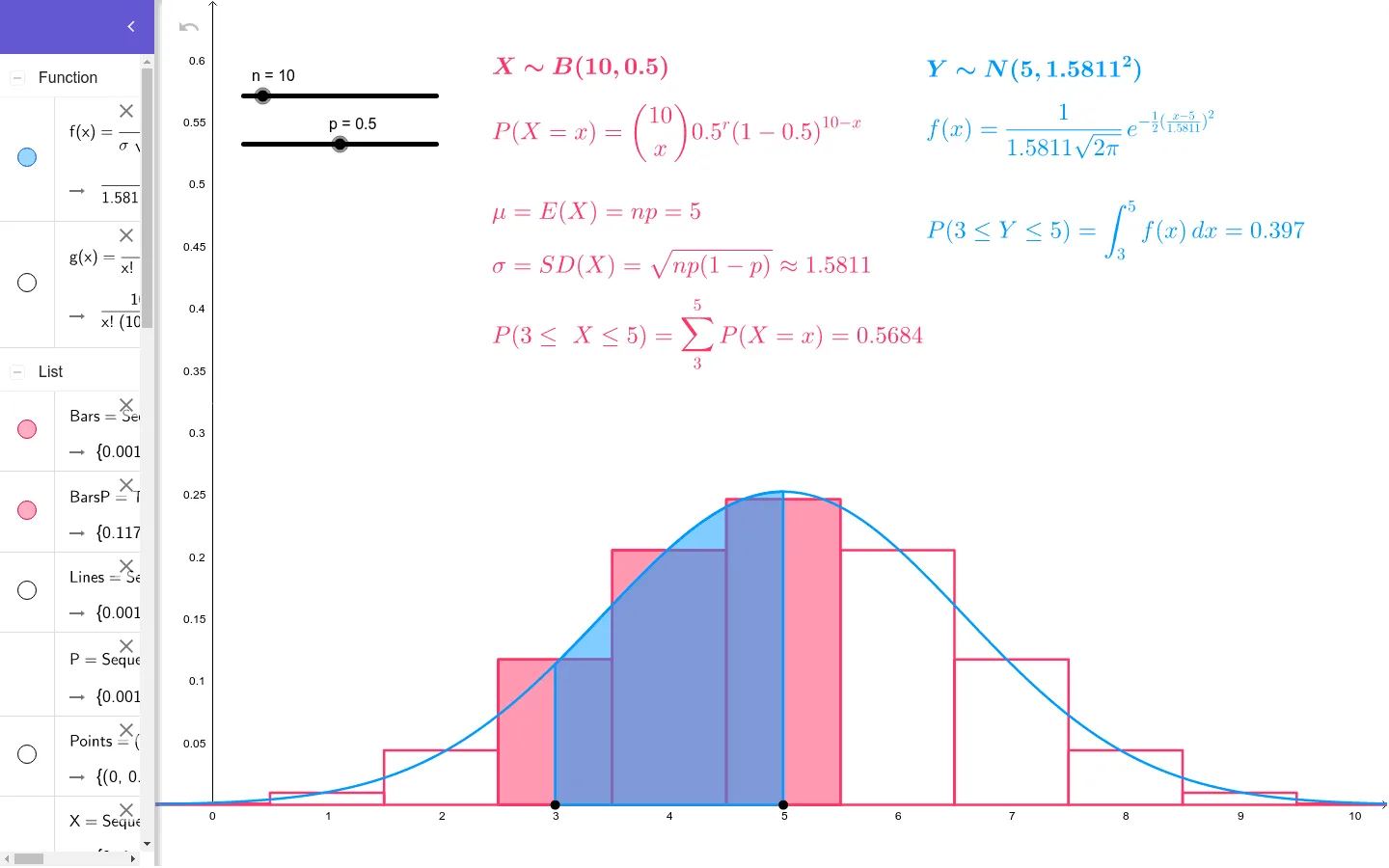
This example demonstrates the relationship between binomial and normal distributions. Key mathematical concepts include probability and statistics, specifically binomial and normal distributions. Using GeoGebra commands like Sequence and NIntegral, dynamic displays of distribution curves for different parameters are shown. Suitable for high school and above students or teachers to understand basic principles of probability and statistics.
GeoGebra Commands & Parameters
Point(xAxis) → APoint(xAxis) → BMax(x(A), x(B)) → bSequence(((nCr[n, r] * p^(r)) * (1 - p)^(n - r)), r, 0, n) → PSequence(k, k, 0, n) → XMin(x(A), x(B)) → aSequence(Segment[(i, 0), (i, g(i))], i, 0, n, 1) → LinesSequence(Polygon[(i - 0.5, 0), (i + 0.5, 0), (i + 0.5, g(i)), (i - 0.5, g(i))], i, 0, n, 1) → BarsIf(b < n, floor(b), n) → b'If(a > 0, ceil(a), 0) → a'Take(Bars, a' + 1, b' + 1) → BarsPNIntegral(f, a, b) → NP
AI Drawing Prompt Reference
Plot the relationship between binomial and normal distributions. Start by creating two points on the x-axis, A and B, and determine the maximum value b and minimum value a. Then generate a sequence of binomial distribution probability values P and corresponding x values X. Next, draw a series of line segments and rectangles to represent the binomial distribution probability bars. Finally, select a portion of the bars based on b and n values and calculate the area under these bars to approximate the area under the normal distribution curve.
The prompt above was compiled from the original drawing commands and is for reference only.