
Binomial Distribution (Dynamic View Window)
Loading the math board and drawing, please wait…
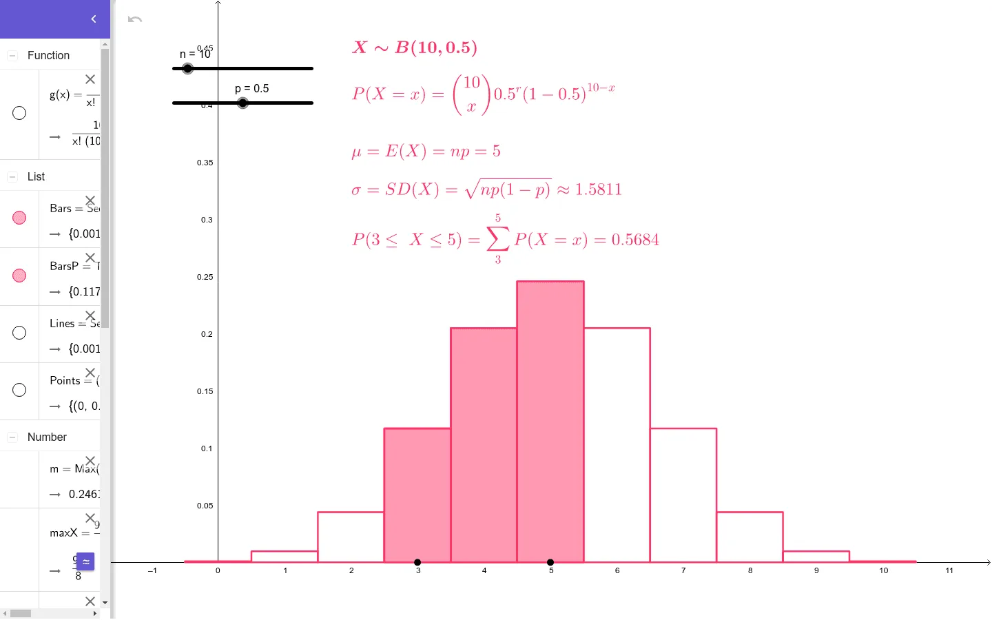
This example demonstrates the binomial distribution. Key mathematical concepts include binomial distribution and probability statistics. Using GeoGebra commands such as Point, Sequence, and If, it dynamically shows the binomial probability density function. Suitable for high school and above students or teachers.
GeoGebra Commands & Parameters
Point(xAxis) → APoint(xAxis) → BMax(x(A), x(B)) → bSequence(((nCr[n, r] * p^(r)) * (1 - p)^(n - r)), r, 0, n) → PSequence(k, k, 0, n) → XMin(x(A), x(B)) → aSequence(Segment[(i, 0), (i, g(i))], i, 0, n, 1) → LinesSequence(Polygon[(i - 0.5, 0), (i + 0.5, 0), (i + 0.5, g(i)), (i - 0.5, g(i))], i, 0, n, 1) → BarsIf(b < n, floor(b), n) → b'If(a > 0, ceil(a), 0) → a'Take(Bars, a' + 1, b' + 1) → BarsPMax(Lines) → m
AI Drawing Prompt Reference
Draw a dynamic graph showing the binomial distribution. Include two points on the horizontal axis, and determine the display range based on their x-coordinates. Use a sequence from 0 to n to calculate the binomial distribution probability at each position, and draw corresponding line segments and bars. The bars start at position a' and end at b', and the line segments connect the heights at each position. Dynamically adjust the display range and probability values.
The prompt above was compiled from the original drawing commands and is for reference only.