
Visualizing Solids of Revolution and Volumes
Loading the math board and drawing, please wait…
In collections
Visualizing Solids of Revolution and Volumes
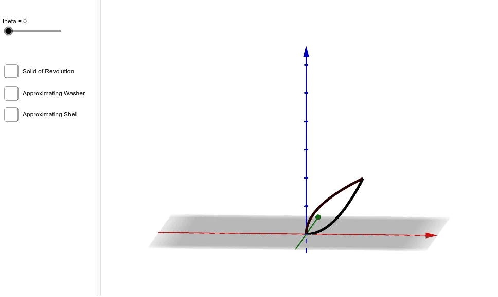
This applet demonstrates the solid of revolution generated by revolving the region bounded by f(x)=√x and g(x)=x around the x-axis. Key mathematical concepts include solids of revolution and volume calculation. It uses commands like Polygon, CurveCartesian, and Surface in GeoGebra. Suitable for high school math education, it helps students understand the process of generating solids of revolution and calculating their volumes.
GeoGebra Commands & Parameters
Polygon((0.5^(2), 0, 0.5), (0.5^(2), 0, 0.6), (sqrt(0.5), 0, 0.6), (sqrt(0.5), 0, 0.5)) → washerpoly, e, f, g, hPolygon(((0.5 * cos(theta)), (0.5 * sin(theta)), 0.5^(2)), ((0.6 * cos(theta)), (0.6 * sin(theta)), 0.5^(2)), ((0.6 * cos(theta)), (0.6 * sin(theta)), sqrt(0.5)), ((0.5 * cos(theta)), (0.5 * sin(theta)), sqrt(0.5))) → shellpolyrev, a, b, c, dPolygon(((0.5^(2) * cos(theta)), (0.5^(2) * sin(theta)), 0.5), ((0.5^(2) * cos(theta)), (0.5^(2) * sin(theta)), 0.6), ((sqrt(0.5) * cos(theta)), (sqrt(0.5) * sin(theta)), 0.6), ((sqrt(0.5) * cos(theta)), (sqrt(0.5) * sin(theta)), 0.5)) → washerpolyrev, i, j, k, lCurveCartesian(t, 0, sqrt(t), t, 0, 1) → topcurveCurveCartesian((t * cos(theta)), (t * sin(theta)), t^(2), t, 0, 1) → fncurverevCurveCartesian(t, 0, t^(2), t, 0, 1) → fncurveCurveCartesian((t * cos(theta)), (t * sin(theta)), sqrt(t), t, 0, 1) → topcurverev_1Surface((0.5 * cos(s)), (0.5 * sin(s)), t, t, 0.5^(2), sqrt(0.5), s, 0, theta) → shellinsiderevSurface((0.6 * cos(s)), (0.6 * sin(s)), t, t, 0.5^(2), sqrt(0.5), s, 0, theta) → shelloutsiderevSurface((t * cos(s)), (t * sin(s)), 0.5^(2), t, 0.5, 0.6, s, 0, theta) → shellbottomrevSurface((t * cos(s)), (t * sin(s)), t^(2), t, 0, 1, s, 0, theta) → bottomcurverevSurface((t * cos(s)), (t * sin(s)), sqrt(t), t, 0, 1, s, 0, theta) → topcurverevSurface((t * cos(s)), (t * sin(s)), 0.5, t, 0.5^(2), sqrt(0.5), s, 0, theta) → washerbottomSurface((t * cos(s)), (t * sin(s)), 0.6, t, 0.5^(2), sqrt(0.5), s, 0, theta) → washertopSurface((sqrt(0.5) * cos(s)), (sqrt(0.5) * sin(s)), t, t, 0.5, 0.6, s, 0, theta) → washeroutsideSurface((0.5^(2) * cos(s)), (0.5^(2) * sin(s)), t, t, 0.5, 0.6, s, 0, theta) → washerinsideSurface((t * cos(s)), (t * sin(s)), sqrt(0.5), t, 0.5, 0.6, s, 0, theta) → shelltoprevPolygon((0.5, 0, 0.5^(2)), (0.6, 0, 0.5^(2)), (0.6, 0, sqrt(0.5)), (0.5, 0, sqrt(0.5))) → shellpoly, p, q, r, s