
Limits in 3D: Visualizing Convergence in Space
Loading the math board and drawing, please wait…
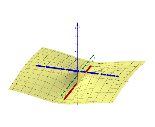
This example demonstrates how to interpret limits in a 3D setting by visualizing geometric objects that approach a target configuration in space. The key mathematical ideas include the concept of a limit (describing behavior as variables get closer to a specified value), representing functional relationships in 3D, and using geometric constructions—such as key points, circles, and constraints—to build an intuitive explanation. From the construction summary, the model is built using GeoGebra objects and relationships: a function f is defined, eq1 provides the governing equation/condition for the configuration, points A and B mark essential positions in the 3D scene, a circle c supports the geometric structure (e.g., representing a cross-section or distance-based locus), and text1 adds labels to emphasize the approaching process. It is well-suited for advanced high school students and early university calculus learners who want to connect limit concepts with solid-geometry visualization.
GeoGebra Commands & Parameters
f(x, y) = (x^(2) - y^(2)) / ((2 * x^(2)) + y^(2))y = 0Numeric c(0.3)(0, c, f(0, c))(c, 0, f(c, 0))
AI Drawing Prompt Reference
Create a 3D surface plot of the function z equals x squared minus y squared divided by two times x squared plus y squared. Mark two special points in the coordinate system: one positioned along the positive y-axis at a distance of 0.3 from the origin, and another along the positive x-axis at the same distance, each displaying their corresponding z-coordinate values. These two points represent function values approached from different directions toward the origin, illustrating the geometric meaning of limits in three-dimensional space.
The prompt above was compiled from the original drawing commands and is for reference only.