
Visualizing Riemann Sum Value Locations
Loading the math board and drawing, please wait…
In collections
Fun with Functions
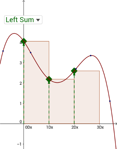
This GeoGebra example dynamically illustrates how different choices of rectangle heights in a Riemann sum—left endpoints, right endpoints, lower sums, upper sums—affect the approximation of a definite integral. The core mathematical concepts include the Riemann sum definition of the integral, left/right sums, lower/upper sums, and the limiting process as the number of subintervals increases. Construction highlights: it uses GeoGebra commands such as RectangleSum, LowerSum, UpperSum to generate rectangles, a slider (n) to control the partition count, Point, Zip, Sort to build rectangle vertices, SelectedIndex and If to switch between sampling strategies, and Vector and Polynomial to display the function curve and rectangle relationships. This resource is ideal for high school or early college calculus students to grasp the geometric meaning of Riemann sums, and for instructors to demonstrate in class, helping learners overcome the common difficulty of visualizing left versus right sums.
GeoGebra Commands & Parameters
SelectedIndex(slist) → indexIf(index ≟ 1, 0, If[index ≟ 2, 0.5, If[index ≟ 3, 1, where]]) → xwPolynomial({C, D, E, F, G}) → gPoint(xAxis) → BPoint(xAxis) → AUpperSum(g, 0, 3, 3) → uppersumRemoveUndefined({(0, g(0)), Extremum[g, 0, 1], (1, g(1))}) → ext0RemoveUndefined({(1, g(1)), Extremum[g, 1, 2], (2, g(2))}) → ext1RemoveUndefined({(2, g(2)), Extremum[g, 2, 3], (3, g(3))}) → ext2Zip(y(a), a, ext0) → ymm0Zip(y(a), a, ext1) → ymm1Zip(y(a), a, ext2) → ymm2Sort(ext0, ymm0) → mm0Sort(ext1, ymm1) → mm1Sort(ext2, ymm2) → mm2RectangleSum(g, 0, 3, 3, xw) → rsumLowerSum(g, 0, 3, 3) → lowersumPoint(pntlist) → JVector(A0, J) → vPoint(pntlist) → KVector(A1, K) → wPoint(pntlist) → LVector(A2, L) → aZip((x(a), 0), a, maxlist) → XmaxlistPoint(Xmaxlist) → HPoint(maxlist) → IVector(H, I) → uPoint(Xmaxlist) → OPoint(maxlist) → PVector(O, P) → cPoint(Xmaxlist) → QPoint(maxlist) → RVector(Q, R) → dZip((x(a), 0), a, minlist) → XminlistPoint(Xminlist) → MPoint(minlist) → NVector(M, N) → bPoint(Xminlist) → SPoint(minlist) → TVector(S, T) → ePoint(Xminlist) → UPoint(minlist) → VVector(U, V) → h