
Visualization of Gravitational Field via Geometric Construction
Loading the math board and drawing, please wait…
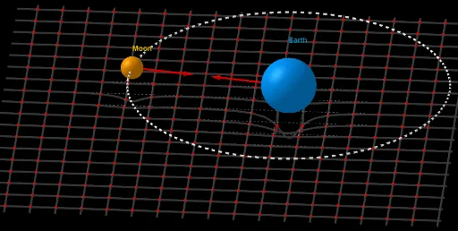
This example visualizes a gravitational field in three‑dimensional space by constructing spheres and vectors that represent the direction and magnitude of the force. It illustrates core concepts such as sphere construction, vector fields, exponential decay, secant lines, and logical combinations. The GeoGebra construction uses commands like Point, Circle, Ray, Sphere, Segment, Intersect, Midpoint, Vector, and Sequence to generate dynamic spheres and vectors, and combines them with logical operations for a rich gravitational distribution. It is intended for high‑school and college students studying spatial geometry, vector calculus, and interdisciplinary STEM topics.
GeoGebra Commands & Parameters
Point(zAxis) → MCircle(M, d_1, zAxis) → cPoint(c) → P_1Ray(P_1, M) → strSphere(P_1 + (0, 0, 1.5), (1.5 * cbrt(m_1))) → k_1Circle(P_1 + (0, 0, 1.5), Distance[P_2, P_1], zAxis) → dSphere(P_2 + (0, 0, 1.5), cbrt(m_2)) → k_2Segment(P_1 + (0, 0, 1.5), P_2 + (0, 0, 1.5)) → f_1Intersect(f_1, k_2) → A,Intersect(f_1, k_1) → B,Midpoint(f_1) → CMidpoint(B, C) → DMidpoint(D, C) → EMidpoint(C, A) → FMidpoint(C, F) → GVector(A, G) → vMidpoint(E, C) → HVector(B, C) → uSequence(Sequence[(i, j, f(i, j)), i, -14, 18, 2], j, -16, 18, 2) → l2