
Visualization of Equivalent Fractions
Loading the math board and drawing, please wait…
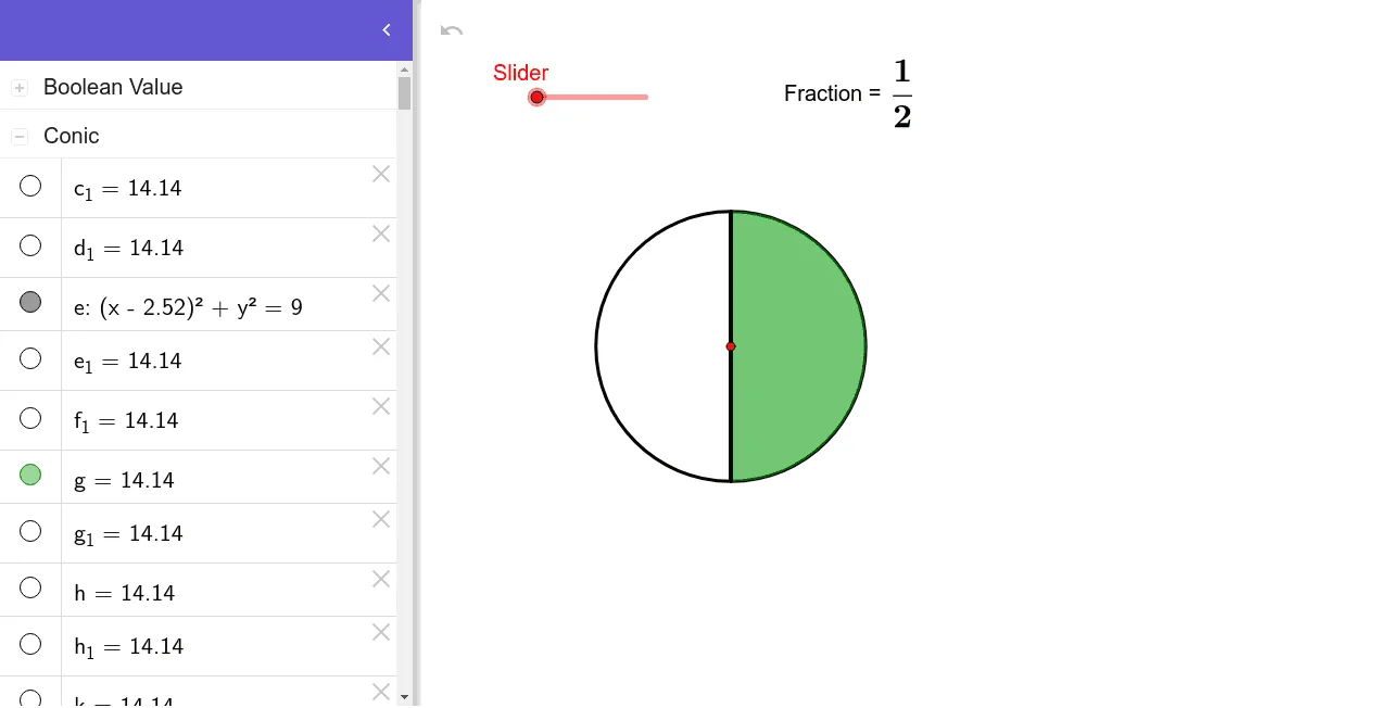
This example dynamically demonstrates the geometric representation of equivalent fractions. It involves core math concepts like fractions, geometric visualization, and similar triangles. Constructed using commands such as Point, Circle, OrthogonalLine, Intersect, Rotate, CircleSector, Segment, Vector, Translate, Polygon, and Slider for interactive learning. Suitable for middle school and above, focusing on visualizing fraction relationships.
GeoGebra Commands & Parameters
Point(xAxis) → ACircle(A, 3) → eOrthogonalLine(A, xAxis) → fIntersect(e, f, 2) → CRotate(C, (360 * ° / Slider), A) → C'Rotate(C', (360 * ° / Slider), A) → C''Rotate(C'', (360 * ° / Slider), A) → C'''Rotate(C''', (360 * ° / Slider), A) → DRotate(D, (360 * ° / Slider), A) → D'Rotate(D', (360 * ° / Slider), A) → D''Rotate(D'', (360 * ° / Slider), A) → D'''Rotate(D''', (360 * ° / Slider), A) → ERotate(E, (360 * ° / Slider), A) → E'Rotate(E', (360 * ° / Slider), A) → E''Rotate(E'', (360 * ° / Slider), A) → E'''Rotate(E''', (360 * ° / Slider), A) → FRotate(F, (360 * ° / Slider), A) → F'Rotate(F', (360 * ° / Slider), A) → F''Rotate(F'', (360 * ° / Slider), A) → F'''Rotate(F''', (360 * ° / Slider), A) → GRotate(G, (360 * ° / Slider), A) → G'Rotate(G', (360 * ° / Slider), A) → G''Rotate(G'', (360 * ° / Slider), A) → G'''CircleSector(A, C, C') → gCircleSector(A, C', C'') → hCircleSector(A, C'', C''') → kCircleSector(A, C''', D) → pCircleSector(A, D, D') → qCircleSector(A, D', D'') → rCircleSector(A, D'', D''') → sCircleSector(A, D''', E) → tCircleSector(A, E, E') → c_1CircleSector(A, E', E'') → d_1CircleSector(A, E'', E''') → e_1CircleSector(A, E''', F) → f_1CircleSector(A, F, F') → g_1CircleSector(A, F', F'') → h_1CircleSector(A, F'', F''') → k_1CircleSector(A, F''', G) → p_1CircleSector(A, G, G') → q_1CircleSector(A, G', G'') → r_1CircleSector(A, G'', G''') → s_1CircleSector(A, G''', C) → t_1Segment(A, C) → iSegment(A, C') → jSegment(A, C'') → lSegment(A, C''') → mSegment(A, D) → nSegment(A, D') → a_1Segment(A, D'') → b_1Segment(A, D''') → i_1Segment(A, E) → j_1Segment(A, E') → l_1Segment(A, E'') → m_1Segment(A, E''') → n_1Segment(A, F) → a_2Segment(A, F') → b_2Segment(A, F'') → c_2Segment(A, F''') → d_2Segment(A, G) → e_2Segment(A, G') → f_2Segment(A, G'') → g_2Segment(A, G''') → h_2Intersect(e, xAxis, 1) → HIntersect(e, xAxis, 2) → IOrthogonalLine(H, xAxis) → i_2OrthogonalLine(I, xAxis) → j_2OrthogonalLine(J, i_2) → k_2OrthogonalLine(K, i_2) → l_2Intersect(j_2, k_2) → LIntersect(j_2, l_2) → MSegment(J, L) → m_2Segment(K, M) → n_2Segment(K, J) → p_2Segment(M, L) → q_2Vector(J, L) → uTranslate(i_2, Vector[u / Slider]) → r_2Translate(i_2, Vector[(u * 2 / Slider)]) → s_2Translate(i_2, Vector[(u * 18 / Slider)]) → t_2Translate(i_2, Vector[(u * 19 / Slider)]) → a_3Translate(i_2, Vector[(u * 17 / Slider)]) → b_3Translate(i_2, Vector[(u * 16 / Slider)]) → c_3Translate(i_2, Vector[(u * 15 / Slider)]) → d_3Translate(i_2, Vector[(u * 14 / Slider)]) → e_3Translate(i_2, Vector[(u * 13 / Slider)]) → f_3Translate(i_2, Vector[(u * 12 / Slider)]) → h_3Translate(i_2, Vector[(u * 11 / Slider)]) → i_3Translate(i_2, Vector[(u * 10 / Slider)]) → j_3Translate(i_2, Vector[(u * 9 / Slider)]) → k_3Translate(i_2, Vector[(u * 8 / Slider)]) → l_3Translate(i_2, Vector[(u * 7 / Slider)]) → m_3Translate(i_2, Vector[(u * 6 / Slider)]) → n_3Translate(i_2, Vector[(u * 5 / Slider)]) → p_3Translate(i_2, Vector[(u * 4 / Slider)]) → q_3Translate(i_2, Vector[(u * 3 / Slider)]) → r_3Intersect(r_2, n_2) → NIntersect(r_2, m_2) → OIntersect(s_2, m_2) → PIntersect(r_3, m_2) → QIntersect(q_3, m_2) → RIntersect(p_3, m_2) → SIntersect(n_3, m_2) → TIntersect(m_3, m_2) → UIntersect(l_3, m_2) → VIntersect(k_3, m_2) → WIntersect(j_3, m_2) → ZIntersect(i_3, m_2) → A_1Intersect(h_3, m_2) → B_1Intersect(m_2, f_3) → D_1Intersect(e_3, m_2) → E_1Intersect(d_3, m_2) → F_1Intersect(c_3, m_2) → G_1Intersect(b_3, m_2) → H_1Intersect(t_2, m_2) → I_1Intersect(a_3, m_2) → J_1Intersect(a_3, n_2) → K_1Intersect(t_2, n_2) → L_1Intersect(b_3, n_2) → M_1Intersect(c_3, n_2) → N_1Intersect(d_3, n_2) → O_1Intersect(e_3, n_2) → P_1Intersect(n_2, h_3) → R_1Intersect(i_3, n_2) → S_1Intersect(j_3, n_2) → T_1Intersect(k_3, n_2) → U_1Intersect(l_3, n_2) → V_1Intersect(m_3, n_2) → W_1Intersect(n_3, n_2) → Z_1Intersect(p_3, n_2) → A_2Intersect(q_3, n_2) → B_2Intersect(r_3, n_2) → C_2Intersect(s_2, n_2) → D_2Intersect(f_3, n_2) → C_1Polygon(J, O, N, K) → poly1, j_4, o, n_4, k_4Polygon(N, D_2, P, O) → poly2, n_5, d_4, p_4, o_1Polygon(D_2, C_2, Q, P) → poly3, d_5, c_4, q_4, p_5Polygon(C_2, B_2, R, Q) → poly4, c_5, b_4, r_4, q_5Polygon(A_2, B_2, R, S) → poly5, a_4, b_5, r_5, s_3Polygon(A_2, Z_1, T, S) → poly6, a_5, z_1, t_3, s_4Polygon(Z_1, W_1, U, T) → poly7, z_2, w_1, u_1, t_4Polygon(W_1, V_1, V, U) → poly8, w_2, v_1, v, u_2Polygon(V_1, U_1, W, V) → poly9, v_2, u_3, w, v_3Polygon(U_1, T_1, Z, W) → poly10, u_4, t_5, z, w_3Polygon(T_1, S_1, A_1, Z) → poly11, t_6, s_5, a_6, z_3Polygon(S_1, R_1, B_1, A_1) → poly12, s_6, r_6, b_6, a_7Polygon(R_1, C_1, D_1, B_1) → poly13, r_7, c_6, d_6, b_7Polygon(C_1, P_1, E_1, D_1) → poly14, c_7, p_6, e_4, d_7Polygon(P_1, O_1, F_1, E_1) → poly15, p_7, o_2, f_4, e_5Polygon(O_1, N_1, G_1, F_1) → poly16, o_3, n_6, g_3, f_5Polygon(M_1, N_1, G_1, H_1) → poly17, m_4, n_7, g_4, h_4Polygon(M_1, L_1, I_1, H_1) → poly18, m_5, l_4, i_4, h_5Polygon(L_1, K_1, J_1, I_1) → poly19, l_5, k_5, j_5, i_5Polygon(K_1, M, L, J_1) → poly20, k_6, m_6, l_6, j_6
AI Drawing Prompt Reference
Draw a circle and create a horizontal line from its center. Find a point on the circle that intersects the line at a certain angle. Rotate this point around the center multiple times, with each rotation angle controlled by a slider, forming several sectors. Connect the center to these points with line segments to display the sector areas, visually demonstrating the geometric representation of fractions and rotational relationships.
The prompt above was compiled from the original drawing commands and is for reference only.