
Unit Circle to Sine and Cosine Functions
Loading the math board and drawing, please wait…
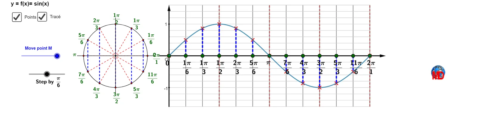
① This interactive GeoGebra example dynamically links a moving point on the unit circle to the graphs of sine and cosine functions, visually demonstrating how the angle determines the function values. ② Core mathematical concepts include the unit circle definition of trigonometric functions, sine and cosine, angle measurement in radians, periodic behavior, and function graphing. ③ Construction highlights: using GeoGebra commands such as Point, Circle, Segment, Vector, Angle, Sequence, Element, List, and Text to build the circle, radius vector, angle display, and point lists; a slider controls the angle parameter to animate the correspondence between the circle and the function graphs. ④ Suitable for high school trigonometry classes, college precalculus review, and anyone seeking an intuitive grasp of how sine and cosine arise from circular motion.
GeoGebra Commands & Parameters
Point(xAxis) → CText("2π", (6.28319, -0.2)) → text2Text("π", (3.141592653589793, -0.2)) → text1Circle(C, 1) → cSegment(C + (1.2, 0), C - (1.2, 0)) → aSequence(Rotate[C + (1, 0), (i * π / n), C], i, 0, (2 * n)) → list4sSegment(C + (0, 1.2), C - (0, 1.2)) → bSequence((i, 0), i, 0, 6.283185307179586, π / n) → list3sSequence(Segment[Element[list4s, i], (x(Element[list4s, i]), 0)], i, 1, k - 1) → list5Sequence(Segment[Element[list4s, i], C], i, 1, k - 1) → list6Segment(Element[list4s, k], C) → dSegment(Element[list4s, k], (x(Element[list4s, k]), 0)) → eElement(list4s, k) → EVector(E, D) → wAngle(Element[list4s, 1], C, E) → αText("x", Element[list3s, k] + (0, -0.2)) → text3Element(list3s, k) → FSegment(D, F) → fVector((-0.3, 0), (6.783185307179586, 0)) → uVector((0, -1.6), (0, 1.6)) → vSequence(Segment[(((i - 1) * π / n), 0), (((i - 1) * π / n), y(Element[list4s, i]))], i, 1, k - 1) → list7Sequence(Segment[((i * π / 2), -1.6), ((i * π / 2), 1.6)], i, 1, 4) → list10Point(list4s) → GSegment(Element[list4s, k], D) → jSequence((((i - 1) * π / n), y(Element[list4s, i])), i, 1, k - 1) → list8sSequence(Segment[((i * π / n), -1.6), ((i * π / n), 1.6)], i, 0, (2 * n)) → list2Sequence(Segment[(0, i), ((2 * π), i)], i, -1.6, 1.6, 0.2) → list1Sequence((i, -1.6), i, 0, 6.28319, π / n) → liste3Sequence(Text["" + (i - 1) + " π / " + n, (x(Element[liste3, i]) - 0.2, y(Element[liste3, i]) - 0.2)], i, 2, k) → liste4Take(liste4, k, k) → liste5Sequence((((i - 1) * π / n), -1.6), i, 1, k) → liste2Text("π/2", (1.5707963267948966, -0.2)) → texte2Text("3π/2", (4.71238898038469, -0.2)) → texte3Sequence(Text["" + (i - 1) + " π / " + n, (x(Element[liste3, i]) - 0.1, y(Element[liste3, i]) - 0.2)], i, 2, k) → liste6Sequence(Text["" + (k) + " π / " + n, C - (0.12, 0) + (1 + 0.25; (k * π / n))], k, 0, (2 * n) - 1, 2) → liste1bSequence(Text["" + (i) + " π / " + n, C - (0.12, 0) + (1 + 0.25; (i * π / n))], i, 0, k - 1, 1) → liste1Element(list4s, k) → MSequence((((i - 1) * π / n), x(Element[list4s, i]) + 1.68), i, 1, k - 1) → liste8cSegment(C, (x(Element[list4s, k]), 0)) → lSegment(Element[list4s, k], (x(Element[list4s, k]), 0)) → mSequence(Segment[(((i - 1) * π / n), 0), (((i - 1) * π / n), y(Element[liste8c, i]))], i, 1, k - 1) → liste7Sequence(Segment[Element[list4s, i], (x(C), y(Element[list4s, i]))], i, 1, k) → l1Sequence((((i - 1) * π / n), 0), i, 1, k - 1) → l4Sequence(Text[If[i ≟ 0, "0", If[i ≟ 4, "π", "\frac{" + (i / GCD[i, 4]) + ((π * "}{") + (4 / GCD[i, 4]) + "}")]], Element[list4s, i], true, true], i, 0, k) → l3Sequence(Text[If[i ≟ 0, "0", If[i ≟ n, "π", "\frac{" + (i / GCD[i, n]) + ((π * "}{") + (n / GCD[i, n]) + "}")]], Element[l4, i + 1] - (0.15, 0.1), true, true], i, 0, (2 * n) + 1) → l5Sequence(Text[If[i ≟ 0, "0", If[i ≟ n, "π", "\frac{" + (i / GCD[i, n]) + ((π * "}{") + (n / GCD[i, n]) + "}")]], C - (0.12, -0.125) + (1 + 0.25; (i * π / n)), true, true], i, 0, (2 * n)) → l2
AI Drawing Prompt Reference
Draw a unit circle and move a point on it to show the angle. Dynamically plot the sine and cosine functions based on the position of this point on the circle. First, draw the unit circle, then place a movable point on it to determine the sine and cosine values based on the angle, and finally plot the graphs of these functions in the coordinate system.
The prompt above was compiled from the original drawing commands and is for reference only.