
Trefoil Knot Parametric Curve
Loading the math board and drawing, please wait…
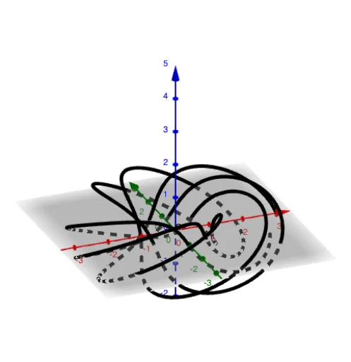
① This example demonstrates a classic trefoil knot as a 3D parametric curve, showing its three-fold looping structure. ② Core mathematical concepts include parametric equations, 3D coordinate systems, knot theory, and trigonometric function combinations, along with transformations between spherical and Cartesian coordinates. ③ Construction details: The GeoGebra command CurveCartesian is used, with parameters a, b, c, n, scale factor, and initial point coordinates (x_0, y_0, z_0) defining the curve; sliders allow dynamic adjustment of shape. ④ Suitable for high school to undergraduate mathematics, useful for teaching analytic geometry, calculus, or introductory topology, helping students understand how parametric equations generate complex spatial curves and how parameter changes affect topological properties.
GeoGebra Commands & Parameters
CurveCartesian(((scale + cos((f * t))) * cos(t) / a) + x_0, ((scale + cos((f * t))) * sin(t) / b) + y_0, sin((f * t)) + z_0, t, 0, ((n * 2) * π)) → c
AI Drawing Prompt Reference
Draw a 3D trefoil knot as a parametric curve with three interlocking loops. The curve is defined by parametric equations where the parameter runs from 0 to 6π, creating a threefold symmetric structure. The x and y coordinates are generated by combinations of cosine and sine functions modulated by a frequency term, while the z coordinate follows a sine function, producing a helical intertwining effect. The curve starts at a given point in space and can be adjusted by scaling factors and frequency parameters to change loop size and tightness, as well as by stretching ratios along each axis to alter the overall shape. The curve should appear as a smooth continuous line, suitable for visualizing how parametric equations generate complex spatial curves.
The prompt above was compiled from the original drawing commands and is for reference only.