
Time Series Construction Problems
Loading the math board and drawing, please wait…
In collections
Charts & Graphs
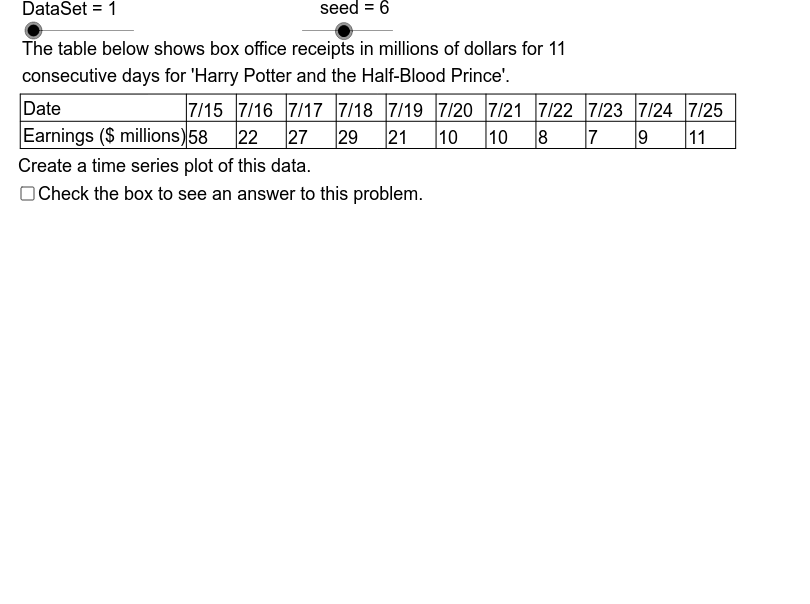
This example demonstrates how to create time series plots using provided data samples and analyze potential solutions. Core math concepts include statistics, histograms, median value, rhombus, centroid, and quadratic equations. GeoGebra commands like Mod, Element, Sequence, Min, Max, Segment, If are used along with objects such as DataSet and Dt series. Suitable for high school students and math enthusiasts learning data analysis and visualization.
GeoGebra Commands & Parameters
Mod(seed, 3) → StrtElement(DtXSq, DataSet) → DtX1Element(DtYSq, DataSet) → DtY1Sequence(Element[DtY1, Strt + k], k, 1, size) → DtY2Min(DtY2) → YMnMax(DtY2) → YMxSequence(Element[DtX1, Strt + k], k, 1, size) → DtX2Segment(Org, GLR) → HAxSegment(Org, GUL) → VAxIf(5 * LBSY ≤ UBSY, 5 * LBSY, If[2 * LBSY ≤ UBSY, 2 * LBSY, LBSY]) → YScl2Sequence(((k - 1) * XScl + GL, AdpY(Element[DtY2, k])), k, 1, size) → DtPtsSequence(Segment[Element[DtPts, k - 1], Element[DtPts, k]], k, 2, size) → GrSgsSegment(TUL, TUR) → TbTpSegment(TLL, TLR) → TbBtSegment(TML, TMR) → TbMdSegment(TLL, TUL) → BLSequence(Text[k, (-3.6, AdpY(k) - 0.35)], k, YAxMn, YAxMx, YScl2) → YLbsSegment((GL - 1.414, GB - 1.414), Org) → LLSgSequence(Segment[(DL + k * CW, TB), (DL + k * CW, TT)], k, 0, size) → DvLnsSequence(Segment[(GL - 0.5, AdpY(k)), (GL + 0.5, AdpY(k))], k, YAxMn, YAxMx, YScl2) → YTcsSequence(Text[Element[DtX2, k], ((k - 1) * XScl + GL - 1, GB - 2.5)], k, 1, size) → XLbsSequence(Segment[(GL + k * XScl, GB - 0.4), (GL + k * XScl, GB + 0.4)], k, 0, size - 1) → XTcsElement(TtlSq, DataSet) → TtlElement(DDSq, DataSet) → DD0Element(VTtlSq, DataSet) → VALblElement(VTtlSq, DataSet) → VATtlElement(TATtlSq, DataSet) → TATtlElement(TATtlSq, DataSet) → TmLblSequence(Text[Element[DtX2, k], (DL - 5.3 + CW * k, TB + 3.5)], k, 1, size) → Rw1Sequence(Text[Element[DtY2, k], (DL - 5.3 + k * CW, TB + 0.5)], k, 1, size) → Rw2
AI Drawing Prompt Reference
Create a time series plot to visualize provided data samples and statistical analysis. Plot data points and connect them to form a time series curve. Calculate and display the minimum and maximum values to define the axis range. Label the axes with appropriate scales and add text annotations. Additionally, draw a rhombus and calculate its centroid to show the central tendency of the data.
The prompt above was compiled from the original drawing commands and is for reference only.