Synthetic Division (Ax−B) Visualization: Track Quotient and Remainder

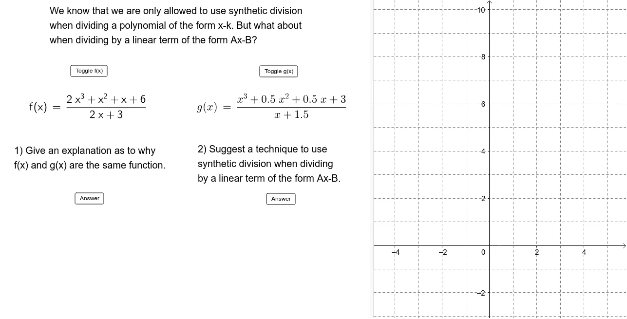
This GeoGebra example visually demonstrates synthetic division for the form (Ax−B), showing how a polynomial is divided by a linear factor using the coefficient-by-coefficient recurrence. It emphasizes the relationship between the process and the quotient polynomial’s coefficients, as well as the remainder that corresponds to evaluating the polynomial at the associated root. Key concepts include polynomial long division via synthetic division, the factor (Remainder) Theorem / linear factor interpretation (remainder equals 0 implies the candidate is a root), and interpreting function or polynomial values to locate roots. Construction details inferred from the setup include multiple function/polynomial objects (f, g), labeled text objects (text1, text2, …, text7) to display intermediate steps and results, geometric points (p, q, r, s) to represent parameter choices or key values, and interactive buttons (button1, button2, button3, button4) to step through the division workflow or toggle inputs. The LaTeX command is used to render the mathematical expressions cleanly, making the coefficient propagation clear. Suitable for secondary-algebra through early university courses, especially for teaching root finding and polynomial division with interactive visualization.