
Surface Between Two Parametric Curves in 3D
Loading the math board and drawing, please wait…
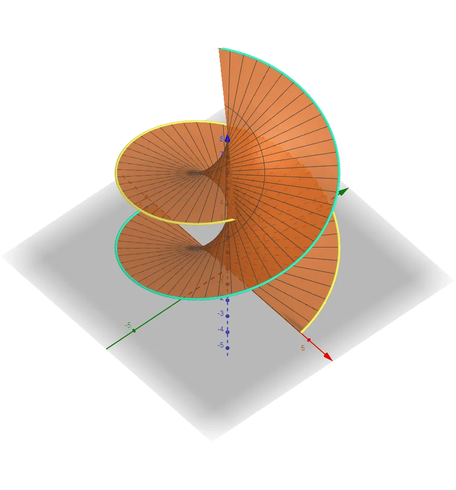
This example demonstrates how to construct a surface in 3D that lies between two parametric curves, revealing how the geometry is smoothly extended from boundary curves into the interior. The key mathematical ideas include parametric equations (parametric curves), surface modeling, and boundary-constrained construction where the two curves act as the upper and lower (or left/right) edges determining the surface. In GeoGebra, the construction is based on using CurveCartesian to define the Cartesian parametric curves (objects such as b, a, c that serve as curve boundaries or supporting curves) and then applying the Surface command to generate the ruled/constructed surface bounded by those curves. Suitable for high school advanced learners and early university students studying analytic geometry, 3D geometry, and parametric representations; also useful for class demonstrations and computational visualization projects.
GeoGebra Commands & Parameters
CurveCartesian(((4.5 * cos(t - π)), (-4.5 * sin(t)), (1.5 * t)), t, 0, (4 * π)) → bCurveCartesian(((4.5 * cos(t)), (4.5 * sin(t)), (1.5 * t)), t, 0, (4 * π)) → aSurface(((1 - u) * a(t)) + (u * b(t)), u, 0, 1, t, 0, (4 * π)) → c
AI Drawing Prompt Reference
Draw a 3D surface defined by two parametric curves. The first curve has x and y varying with cosine and sine, and z increasing linearly with time. The second curve is similar but y changes with opposite sign. The surface extends smoothly from these curves, forming a transition region. The boundary is defined by these curves, and the interior is controlled by a parameter u.
The prompt above was compiled from the original drawing commands and is for reference only.