Quartic Formula Demo: Algebraic Reduction and Geometric Insight

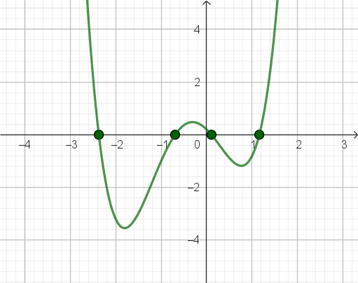
This example demonstrates the structural workflow behind solving a quartic equation, combining algebraic reduction with a GeoGebra construction that makes the parameter dependencies visually traceable. It focuses on the key ideas of quartic solving—using coefficient-driven transformations, reduction to a cubic subproblem, and conditional case handling to select the correct expression—while supporting geometric intuition via related transformation/similarity setup. Core concepts include quartic-to-cubic reduction, polynomial coefficient parametrization (a0, a1, a2, a3), and the use of intermediate discriminant-like quantities (e.g., R, D, E) and root candidates (z1–z4) that are assembled into final expressions. In the construction, SolveCubic is used to compute the cubic step; LaTeX is used to render the symbolic formulas; If provides branching logic for different cases. The construction relies on objects such as λ, p, q, r, g, y1, R, D, E, z1–z4, and lines l1, l2 together with function-like objects f and text annotations for clarity. Suitable for high school honors, early university algebra, and learners who want to visualize how the quartic formula is assembled from intermediate parameters.